Assessing Annotator Disagreements in Python to Build a Robust Dataset for Machine Learning

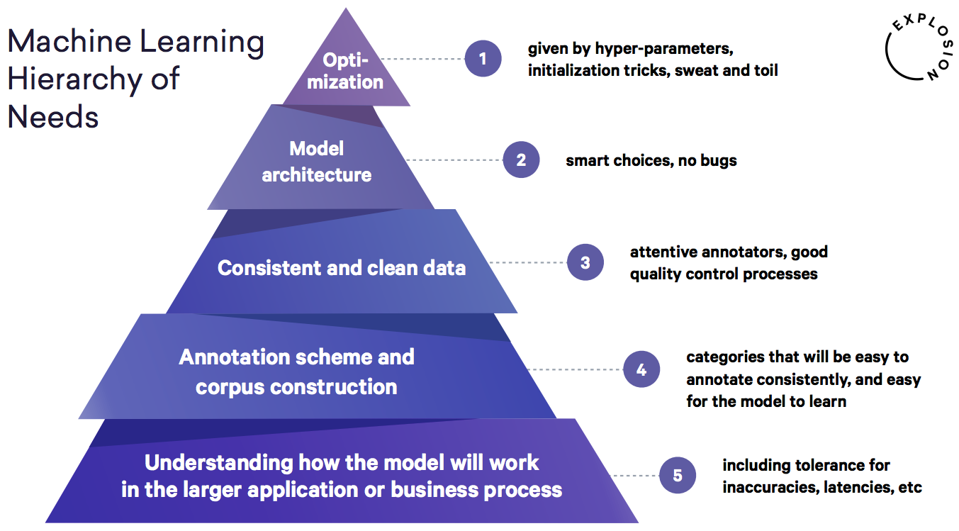
As Matthew Honnibal pointed out at his 2018 PyData Berlin talk [1], developing a solid annotation schema and having attentive annotators is one of the building blocks of a successful machine learning model, and an integral part of the workflow. The pyramid below — taken from his slides — shows these as being essential stages prior to model development.

Having recently completed an MSc in Data Analytics and then working closely with a charity in machine learning, what is only now striking me as troubling about the state of formal education is the distinct under-focus on the bottom three building blocks, and an over-focus on the top two blocks. Despite it being troubling, the reason is clear: students aren’t attracted to the gritty pre-machine learning phase. But the fact remains that without an understanding of how to work on what might be less exciting, it simply won’t be possible to build a robust, strong, and reliable machine learning product.

I’ve noticed that explanations of annotation disagreement assessment methods are not confined to a single post on the web, and methods for doing this in Python are not confined to a single library. So in this post we will cover a number of important topics in the annotator agreements space:

1. Definitions of well-known statistical scores for assessing agreement quality. (The maths can also be found on the relevant Wikipedia pages.)
2. Python implementations of these statistical scores using a new library I wrote, called disagree.
3. How to assess which labels warrant further attention using the same library, introducing the concept of bidisagreements.

What is an annotation schema?

Before we can start doing any form of computational learning, we need a data set. In supervised learning, in order for the computer to learn, each instance of our data must have some label. To obtain the labels, we might need a group of people to sit down and manually label each instance of data — these people are annotators. In order to allow people to do this, we must develop and write an annotation schema, advising them on how to correctly label the instances of data.

When multiple annotators label the same instance of data (as is always the case), there might be disagreements about what the label should be. Disagreements amongst annotators are not good, because it means that we cannot effectively allocate instances with labels. If we begin allocating instances of data with labels for which there was significant disagreement, then our machine learning model is in serious danger. This is because the data cannot be relied on, and neither can any model we develop.

Thus, once the data has all been labelled, it is imperative to investigate these cases of disagreement, so that we can gain knowledge and understanding about where disagreements come from.

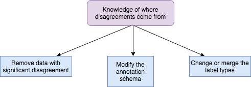
1. Remove data with significant disagreements: This leaves us with only data that has been confidently labelled and is reliable.
2. Modify the annotation schema for future use: It could be that it wasn’t written clearly, and we can improve future agreement.
3. Change or merge the label types: Perhaps we were fundamentally wrong about the types of labels that would be useful. Sometimes we need to modify labels to fit annotator capabilities.

In order to run through a number of the most useful (and not-so-useful) methods for quantitatively evaluating the inter-annotator disagreements, I will first show you how to set up the Python ‘disagree’ library. Then I will go through a variety of statistics, combining both mathematical theory and Python implementations.

The ‘disagree’ library

It aims to do a few things:

1. Provide statistical capabilities for quantitatively assessing annotator disagreements.

2. Provide visualisations between different annotators.

3. Provide visualisations to see which labels experience the most disagreement.

After observing each of these three points, the three solutions mentioned above can be considered if necessary. First, you need to import the library. Below is every module available, all of which I will demonstrate here:

from disagree import BiDisagreementsfrom disagree import Metrics, Krippendorff

There are two nuances fundamental to disagree. The first is that you need the annotations to be stored in a pandas DataFrame in a specific way. The rows are indexed by the instance of data, and the columns are each annotator’s label for that instance of data. The column headings are the annotator’s names as strings. Labels must be either None, or between 0 and the maximum label. (You have to convert your labels to this format.) So let’s set up an example DataFrame so that this is clear:

example_annotations = {"a": [None, None, None, None, None, 1, 3, 0, 1, 0, 0, 2, 2, None, 2], "b": [0, None, 1, 0, 2, 2, 3, 2, None, None, None, None, None, None, None], "c": [None, None, 1, 0, 2, 3, 3, None, 1, 0, 0, 2, 2, None, 3]}

labels = [0, 1, 2, 3]

So in our example we have 3 annotators named “a”, “b”, and “c”, who have collectively labelled 15 instances of data. (The first instance of data is not labelled by “a” and “c”, and is labelled as 0 by “b”.) The dataframe will look like this:

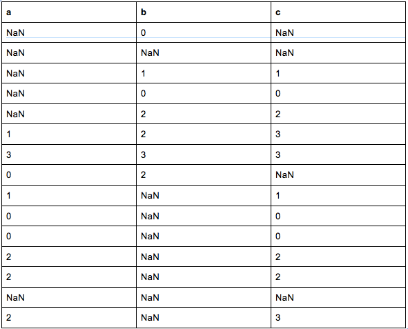
Furthermore, for each instance they had the choice of labels [0, 1, 2, 3]. (In reality, they could have had the choice of [1, 2, 3, 4] or [“cat”, “dog”, “horse”, “cow”], but the labels had to be indexed from zero for use in the library.)

Now we are ready to explore the possible metrics used to assess annotator agreements. Start by setting up the Metrics instance from the metrics module:

mets = metrics.Metrics(df, labels)

Joint Probability

The joint probability is the most simple, and most naïve, method for assessing annotator agreements. It can be used to look at how much one annotator agrees with another.

Essentially, it adds up the number of times annotators 1 and 2 agree, and divides it by the total number of data points that they both labelled.

For our example dataset, we can compute this between two annotators of our choice:

joint_prob = mets.joint_probability("a", "b")

print("Joint probability between annotator a and b: {:.3f}".format(joint_prob))

Out: Joint probability between annotator a and b: 0.333

Cohen’s kappa

This is a more statistically advanced method than joint probability because it considers the probability of agreeing by chance. It also compares two annotators.

Using the Python library:

cohens = mets.cohens_kappa("a", "b")

print("Cohens kappa between annotator a and b: {:.3f}".format(cohens))

Out: Cohens kappa between annotator a and b: 0.330

Correlation

Correlation is also an obvious choice! If annotator 1 and annotator 2 have a high correlation, then they are likely to agree on labels. Conversely, a low correlation means that they are unlikely to agree.

spearman = mets.correlation("a", "b", measure="spearman")pearson = mets.correlation("a", "b", measure="pearson")kendall = mets.correlation("a", "b", measure="kendall")

print("Spearman's correlation between a and b: {:.3f}".format(spearman[0]))print("Pearson's correlation between a and b: {:.3f}".format(pearson[0]))print("Kendall's correlation between a and b: {:.3f}".format(kendall[0]))

Out: Spearman's correlation between a and b: 0.866Out: Pearson's correlation between a and b: 0.945Out: Kendall's correlation between a and b: 0.816

Note that with the correlation measures, a tuple of the correlation and p-value is returned, hence the zero-indexing when printing the result. (This uses the scipy library.)

At this point, you might be thinking the following: “But what if we have more than two annotators? Aren’t these methods pretty useless?” The answer can be both “Yes” and “No”. Yes, they would be useless for assessing global annotator disagreements with respect to making your dataset more robust. However, there are a number of cases when you might want to do this:

• Imagine you have 10 annotators, 2 of which sit in a room together, whilst the other 8 sit separately. (Perhaps due to office space.) Following the annotations, you might want to see if there is greater agreement between the two who sat in a room together, since they might have been discussing the labels.
• Perhaps you want to see the agreement amongst annotators with the same educational background, relative to groups from another educational background.

Now I will go through a number of more advanced — and arguably the most popular — methods for assessing annotator agreement statistics across any number of annotators. These are more commonly seen in modern machine learning literature.

Fleiss’ kappa

Fleiss’ kappa is an extension of Cohen’s kappa. It extends it by considering the consistency of annotator agreements, as opposed to absolute agreements that Cohen’s kappa looks at. This is a statistically reliable method, and is commonly used in the literature to demonstrate data quality.

In Python:

fleiss = mets.fleiss_kappa()

Krippendorff’s alpha

The final, most computationally expensive, and mathematically messy, is Krippendorff’s alpha. This, along with Fleiss’ kappa, is considered one of the most useful statistics (if not the most useful). (There’s a great example on the Wikipedia page if you want to see manual computation of Krippendorph’s alpha.)

In Python, this is as simple as any of the other statistics:

kripp = Krippendorff(df, labels)alpha = kripp.alpha(data_type="nominal")

print("Krippendorff's alpha: {:.3f}".format(alpha))

Out: Krippendorff's alpha: 0.647

The reason I reserve Krippendorff’s alpha for a separate class is because there are a few very computationally expensive processes in the initialisation. If there are a large number of annotations (say, 50,000 to 100,000) it would be frustrating to have to initialise Krippendorff alpha data structures when one is not interested in using it. Having said this, it has been implemented in such a way that it doesn’t take long to run anyway.

And there it is — computing an array of useful annotation disagreement statistics in one easy-to-use, compact Python library.

Bidisagreements

Another useful thing to consider is something I like to call bidisagreements. These are the number of times that an instance of data is labelled differently by two different annotators. The reason these are useful is because they allow you to examine where there might be flaws in the labelling system used, or the annotation schema provided to the annotators.

For example, on a given instance of the dataset, the labels [0, 0, 1], or [1, 1, 1, 2], or [1, 3, 1, 3] would each be considered a single bidisagreement. (Rows 8 and 15 are examples of bidisagreements in the dataframe above.) This can be extended to tridisagreements, 4-disagreements, 5-disagreements, and so on.

Using the disagree library, we can examine these cases with the BiDisagreements module, which was imported above.

First, set up the instance:

bidis = BiDisagreements(df, labels)

A useful attribute is the following:

bidis.agreements_summary()

Number of instances with:=========================No disagreement: 9Bidisagreement: 2Tridisagreement: 1More disagreements: 0Out[14]: (9, 2, 1, 0)

The output shows that from our example annotations, there are 9 instances of data for which there are no disagreements; 2 instances of data for which there is a bidisagreement; and 1 instance of data for which there is a tridisagreement. (Note that this returns the tuple as the output.) The reason these add up to 12 and not 15 is because in our example dataset, there are 3 instances where at most 1 annotator labelled the instance. These are not included in the computations because any instance of data labelled by 1 annotator should be considered void anyway.

We can also visualise which labels are causing the bidisagreements:

mat = bidis.agreements_matrix(normalise=False)print(mat)

[[0. 0. 1. 0.] [0. 0. 0. 0.] [1. 0. 0. 1.]  [0. 0. 1. 0.]]

From this matrix, we can see that one bidisagreement stems from label 0 vs label 2, and the other stems from label 2 vs label 3. Using this matrix, you can create a visualisation of your choice — such as something in the form of a confusion matrix using matplotlib: https://www.kaggle.com/grfiv4/plot-a-confusion-matrix.

This final capability is particularly useful when you have very large datasets. Recently, using this on 25,000 annotations across 6,000 data instances, I was able to very quickly identify that almost 650 bidisagreements were coming from just two labels. This allowed me to address these two labels and how they were to be used in the machine learning model, as well as when modifying the annotation schema for future use by annotators.

Future consideration

With bidisagreements, you will have noticed that the library is only capable of showing the the frequency. This has a somewhat significant floor. Imagine the following two sets of labels for two instances of data:

1. [0, 0, 0, 0, 1]
2. [2, 1, 1, 2, 2]

Clearly, the first one has much better agreement than the second one, yet disagree considers them equally. It will be interesting to work towards a bidisagreement method that statistically weights the second one as a more significant bidisagreement than the first, and then normalises the bidisagreements matrix accordingly.

Final notes about ‘disagree’

This library is very recent, and is my first implementation of one. (For this reason, I ask you to please excuse the messy version and commit histories.) The full GitHub repo can be found here: https://github.com/o-P-o/disagree.

The repo includes all of the code, as well as Jupyter notebooks with the examples illustrated above. There is also a full documentation in the README file.

Please feel free to raise issues and make suggestions for additional capabilities as well. I will address any of these promptly.