At the core of hotel personalization and ranking is the challenge of matching a set of hotels to a set of travelers whose tastes are heterogeneous and sometimes unobserved. The accuracy of the match depends on how online travel agencies (OTA) leverage their available information such as given hotel characteristics, location attractiveness of hotels, users aggregated purchase history and competitors’ information, and among others, to infer travelers preferences for hotels. For example,

Here is our goal today: applying machine learning techniques to maximize the click-through for the presented choices, where a click indicates a visitor’s interest and potentially a decision to book.

Eventually, this is what we want to achieve: when a user inputs his (or her) search criteria into the hotel search engine, a filtered personalized sorted list of available hotels will be shown to him (or her) according to the above ranking algorithm, so that the hotels at the top of the list are the ones with the highest probability of being clicked by the user. And we do this step by step.

Data Description

The data set contains the following information and can be downloaded from Kaggle, and we will use train.csv.

Let’s try to make column names more intuitive.

Data Preprocessing

import pandas as pd

df = pd.read_csv('train.csv')df.shape

(9917530, 54)

This is a large data set with near 10 million observations and 54 features. So, I am looking for a way to make it more manageable.

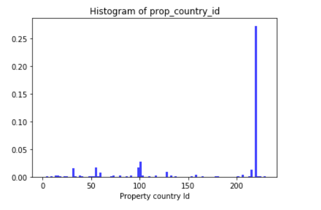
import matplotlib.pyplot as pltn, bins, patches = plt.hist(df.prop_country_id, 100, density = 1, facecolor='blue', alpha=0.75)plt.xlabel('Property country Id')plt.title('Histogram of prop_country_id')plt.show();

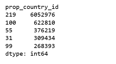
df.groupby('prop_country_id').size().nlargest(5)

n, bins, patches = plt.hist(df.visitor_location_country_id, 100, density = 1, facecolor='blue', alpha=0.75)plt.xlabel('Visitor location country Id')plt.title('Histogram of visitor_location_country_id')plt.show();

df.groupby('visitor_location_country_id').size().nlargest(5)

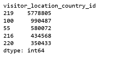
The data is anonymized, so determining the exact country or city to which a consumer plans to travel to is not possible. However, it is evident that the largest country (labeled 219) is the United States. The largest country has 61% of all observations. Out of those, 58% of searches are made by consumers also located in this country, suggesting that the country has a large territory with a large fraction of domestic travel. The price currency also suggested that the largest country being the United States.

Therefore, to improve the computational efficiency, we are going to train independent models on US visitors. This method greatly reduces time on training.

us = df.loc[df['visitor_location_country_id'] == 219]us = us.sample(frac=0.6, random_state=99)del us['visitor_location_country_id']

Limited by computational power, we randomly take 60% of the US data set. Then remove the column “visitor_location_country_id”.

us.isnull().sum()

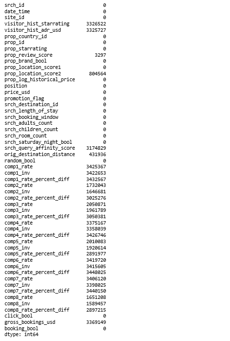
As you can see, we have a lot of missing data in many features. We are going to drop features that have more than 90% of NaN values, also drop “date_time”, “srch_id” and “prop_id”, and impute three features that contain less than 30% of NaN value, they are: “prop_review_score”, “prop_location_score2” and “orig_destination_distance”.

cols_to_drop = ['date_time', 'visitor_hist_starrating', 'visitor_hist_adr_usd', 'srch_query_affinity_score', 'comp1_rate', 'comp1_inv', 'comp1_rate_percent_diff', 'comp2_rate_percent_diff', 'comp3_rate_percent_diff', 'comp4_rate_percent_diff', 'comp5_rate_percent_diff', 'comp6_rate_percent_diff', 'comp7_rate_percent_diff', 'comp8_rate_percent_diff', 'comp2_rate', 'comp3_rate', 'comp4_rate', 'comp5_rate', 'comp6_rate', 'comp7_rate', 'comp8_rate', 'comp2_inv', 'comp3_inv', 'comp4_inv', 'comp5_inv', 'comp6_inv', 'comp7_inv', 'comp8_inv', 'gross_bookings_usd', 'srch_id', 'prop_id']us.drop(cols_to_drop, axis=1, inplace=True)

Randomly impute “prop_review_score”

This method eliminates the imputation variance of the estimator of a mean or total, and at the same time preserves the distribution of item values.

Impute “prop_location_score2” with mean

us['prop_location_score2'].fillna((us['prop_location_score2'].mean()), inplace=True)

Impute “orig_destination_distance” with median

us['orig_destination_distance'].fillna((us['orig_destination_distance'].median()), inplace=True)

We are done with the imputation!

EDA

us.shape

(3467283, 22)

After basic data cleaning, our USA data set contains over 3.4 million observations and 22 features. Let’s explore those features.

Click and book

Our target variable is “click_bool”, rather than “booking_bool”. Because where there is a booking, there must be a click, and we want to optimize clicks.

import matplotlib.pyplot as pltimport seaborn as snssns.countplot(x='booking_bool',data=us, palette='hls')plt.show();

us['booking_bool'].value_counts()

sns.countplot(x='click_bool',data=us, palette='hls')plt.show();

us['click_bool'].value_counts()

Due to the nature of online travel business, both booking rate(2.8%) and click through rate (4.3%) are extremely low, the non-click impressions are overwhelming, the class are very imbalanced.

Search length of stay

n, bins, patches = plt.hist(us.srch_length_of_stay, 50, density = 1, facecolor='blue', alpha=0.75)plt.xlabel('Search length of stay')plt.title('Histogram of search_length_of_stay')plt.axis([0, 30, 0, 0.65])plt.show();

us.groupby('srch_length_of_stay').size().nlargest(5)

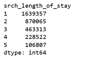
The most searched length_of_stay is 1 day, then 2, 3, … Nothing outlier.

Search adults count

n, bins, patches = plt.hist(us.srch_adults_count, 20, density = 1, facecolor='blue', alpha=0.75)plt.xlabel('Search adults count')plt.title('Histogram of search_adults_count')plt.show();

df.groupby('srch_adults_count').size().nlargest(5)

The most common search adults count is 2-adults, then 1-adult, makes sense.

Property star rating

n, bins, patches = plt.hist(us.prop_starrating, 20, density = 1, facecolor='blue', alpha=0.75)plt.xlabel('Property star rating')plt.title('Histogram of prop_star_rating')plt.show();

The most common searched property star rating is 3 stars. Good to know, I would have thought higher.

Property is a brand or not

us.groupby('prop_brand_bool').size()

More than 73% of the properties are brand properties. It does make sense since we are talking about US hotels and US travelers.

Stay on Saturday or not

us.groupby('srch_saturday_night_bool').size()

Price USD

sns.set(style="ticks", palette="pastel")

ax = sns.boxplot(x="click_bool", y="price_usd", hue="click_bool", data=us)ax.set_ylim([0, 200]);

us.groupby('click_bool')['price_usd'].describe()

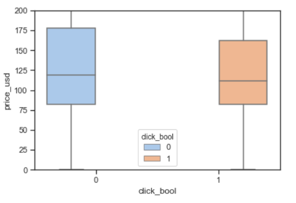
On average, the price_usd that received a click is always lower than those of did not get a click.

Balancing the Classes

For fast learning, our balancing strategy is down sampling negative instances.

Model Training and Evaluation

Click-through prediction with Ensemble models

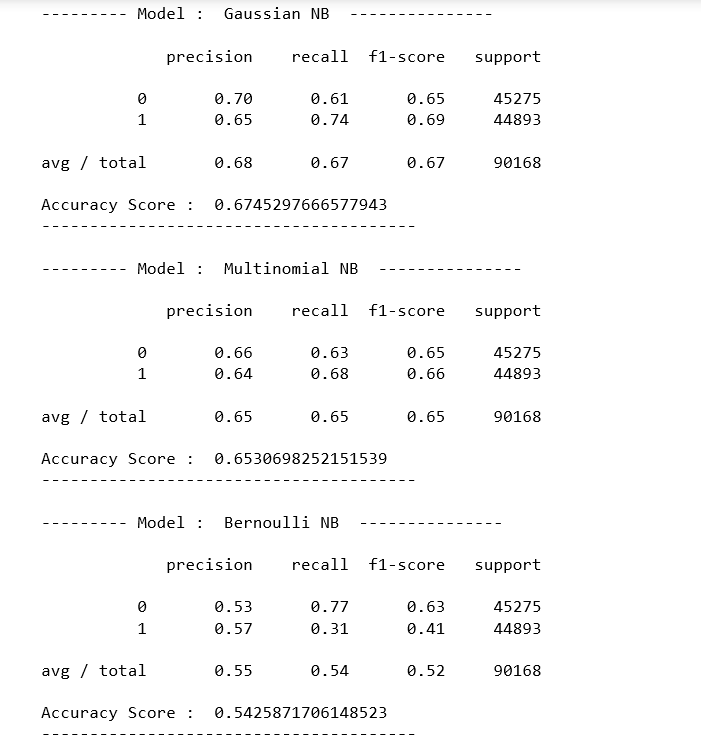
Click-through prediction with Naive Bayes models

Click-through prediction with Neural network

Based on this baseline approach, in the future posts, we will be building a learning to rank model to personalize hotel ranking for each impression. But until then, enjoy clicking!