
CNTK API文件翻譯(9)——使用自編碼器壓縮MNIST資料
在本期教程之前需要先完成第四期教程。
介紹
本教程介紹自編碼器的基礎。自編碼器是一種用於高效編碼的無監督學習人工神經網路,換句話說,自編碼器用於通過機器學習學來的演算法而不是人寫的演算法進行有損資料壓縮。由此而來,使用自編碼器編碼的目的是訓練出一套資料表示方法來編碼或者說表述一個數據集,經常被用於資料降維。
自編碼器非常依賴於不同的資料,他們和傳統的編碼/解碼器比如JPEG,MPEG等非常不同,沒有一個編碼標準。由於是有失真壓縮,因此當一段資料被編碼然後又解碼回去,會有一部分資訊丟失,所以自編碼器基本不會真正用於資料壓縮,缺在兩大領域有奇效:去噪和資料降維。
自編碼器一直默默無聞,直到科學家們發現他在無監督學習上大有可為。真正的無監督學習是完全不需要標記的,不過自編碼器因為可以進行自對照,因此也被叫做自監督學習,也就是把輸入資料當標記的機器學習。
目標
我們的目標是訓練一個自編碼器,把MNIST資料壓縮成一個更小維度的向量,然後再儲存成影象。MNIST是由一些有點背景噪音的手寫數字影象組成的。
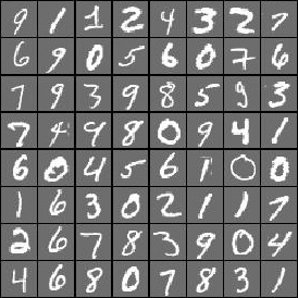
在本教程中,我們會使用MNIST資料來展示使用前饋神經網路編碼和解碼影象。我們會對比編碼前的影象和經過編碼解碼之後的影象。我們會使用前饋神經網路構建簡單自編碼器和深度自編碼器。更多的自編碼器會在以後的教程中涉及到。
# Import the relevant modules
from __future__ import print_function # Use a function definition from future version (say 3.x from 2.7 interpreter) 在下面的程式碼中,我們通過檢查在CNTK內部定義的環境變數來選擇正確的裝置(GPU或者CPU)來執行程式碼,如果不檢查的話,會使用CNTK的預設策略來使用最好的裝置(如果GPU可用的話就使用GPU,否則使用CPU)
# Select the right target device when this notebook is being tested:
if 'TEST_DEVICE' 我們設定了兩種執行模式:
- 快速模式:isFast變數設定成True。這是我們的預設模式,在這個模式下我們會訓練更少的次數,也會使用更少的資料,這個模式保證功能的正確性,但訓練的結果還遠遠達不到可用的要求。
- 慢速模式:我們建議學習者在學習的時候試試將isFast變數設定成False,這會讓學習者更加了解本教程的內容。
資料讀取
在本部分我們將使用第四期下載的資料。資料格式如下:
|labels 0 0 0 1 0 0 0 0 0 0 |features 0 0 0 0 … (784 integers each representing a pixel gray level)
在本期教程中,我們使用代表畫素值的數值串作為特徵值。下面定義create_reader函式來讀取訓練資料和測試資料,程式碼中使用到了CTF(CNTK text-format) Deserializer,標籤使用一位有效編碼。
# Read a CTF formatted text (as mentioned above) using the CTF deserializer from a file
def create_reader(path, is_training, input_dim, num_label_classes):
    return C.io.MinibatchSource(C.io.CTFDeserializer(path, C.io.StreamDefs(
        labels_viz = C.io.StreamDef(field='labels', shape=num_label_classes, is_sparse=False),
        features   = C.io.StreamDef(field='features', shape=input_dim, is_sparse=False)
    )), randomize = is_training, max_sweeps = C.io.INFINITELY_REPEAT if is_training else 1)


# Ensure the training and test data is generated and available for this tutorial.
# We search in two locations in the toolkit for the cached MNIST data set.
data_found = False
for data_dir in [os.path.join("..", "Examples", "Image", "DataSets", "MNIST"),
                 os.path.join("data", "MNIST")]:
    train_file = os.path.join(data_dir, "Train-28x28_cntk_text.txt")
    test_file = os.path.join(data_dir, "Test-28x28_cntk_text.txt")
    if os.path.isfile(train_file) and os.path.isfile(test_file):
        data_found = True
        break

if not data_found:
    raise ValueError("Please generate the data by completing CNTK 103 Part A")
print("Data directory is {0}".format(data_dir))
模型建立
我們首先假設用一個簡單的全連線前饋神經網路來當作編碼器和解碼器(如下圖)。
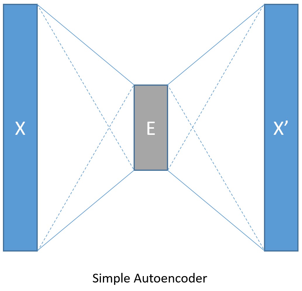
輸入資料使用MNIST的手寫數字影象,每個影象都是28×28畫素。在本教程中,我們把每個影象都當做一個線性陣列,裡面的值就是這784個畫素的畫素值,所以輸入值的大小應該是784。因為我們的目標是先編碼然後解碼,所以輸出的大小應該跟輸入的大小一樣。我們將設定壓縮後的資料大小是32。另外畫素值範圍是0到255,在輸入時需要歸一化成0到1之間。
input_dim = 784
encoding_dim = 32
output_dim = input_dim

def create_model(features):
    with C.layers.default_options(init = C.glorot_uniform()):
        # We scale the input pixels to 0-1 range
        encode = C.layers.Dense(encoding_dim, activation = C.relu)(features/255.0)
        decode = C.layers.Dense(input_dim, activation = C.sigmoid)(encode)

    return decode
訓練和測試
在以前的教程中,我們經常把訓練和測試分成不同的小結,這期我們把他們合在一起,這種方式在以後的實際應用中也可以使用。
train_and_test函式主要執行了如下兩個任務:
- 訓練模型
- 用測試資料評估模型精度
在訓練時:
設定了三個網路的輸入值,分別是reader_train(資料讀取器),model_func(模型函式)和label(標籤)。在本教程中,我們展示瞭如何建立和使用自己的成本函式。如上文所述,我們需要歸一化label函式,讓他的輸出值在0和1之間,方便我們使用C.classification_error來計算差值。
在CNTK提供的一系列訓練器中,我們選擇Adam訓練器。
在測試時:
另外引入了reader_test(測試資料讀取器),用來和通過模型生成的畫素值對比。
def train_and_test(reader_train, reader_test, model_func):

    ###############################################
    # Training the model
    ###############################################

    # Instantiate the input and the label variables
    input = C.input_variable(input_dim)
    label = C.input_variable(input_dim)

    # Create the model function
    model = model_func(input)

    # The labels for this network is same as the input MNIST image.
    # Note: Inside the model we are scaling the input to 0-1 range
    # Hence we rescale the label to the same range
    # We show how one can use their custom loss function
    # loss = -(y* log(p)+ (1-y) * log(1-p)) where p = model output and y = target
    # We have normalized the input between 0-1. Hence we scale the target to same range

    target = label/255.0
    loss = -(target * C.log(model) + (1 - target) * C.log(1 - model))
    label_error  = C.classification_error(model, target)

    # training config
    epoch_size = 30000        # 30000 samples is half the dataset size
    minibatch_size = 64
    num_sweeps_to_train_with = 5 if isFast else 100
    num_samples_per_sweep = 60000
    num_minibatches_to_train = (num_samples_per_sweep * num_sweeps_to_train_with) // minibatch_size


    # Instantiate the trainer object to drive the model training
    lr_per_sample = [0.00003]
    lr_schedule = C.learning_rate_schedule(lr_per_sample, C.UnitType.sample, epoch_size)

    # Momentum
    momentum_as_time_constant = C.momentum_as_time_constant_schedule(700)

    # We use a variant of the Adam optimizer which is known to work well on this dataset
    # Feel free to try other optimizers from
    # https://www.cntk.ai/pythondocs/cntk.learner.html#module-cntk.learner
    learner = C.fsadagrad(model.parameters,
                         lr=lr_schedule, momentum=momentum_as_time_constant)

    # Instantiate the trainer
    progress_printer = C.logging.ProgressPrinter(0)
    trainer = C.Trainer(model, (loss, label_error), learner, progress_printer)

    # Map the data streams to the input and labels.
    # Note: for autoencoders input == label
    input_map = {
        input  : reader_train.streams.features,
        label  : reader_train.streams.features
    }

    aggregate_metric = 0
    for i in range(num_minibatches_to_train):
        # Read a mini batch from the training data file
        data = reader_train.next_minibatch(minibatch_size, input_map = input_map)

        # Run the trainer on and perform model training
        trainer.train_minibatch(data)
        samples = trainer.previous_minibatch_sample_count
        aggregate_metric += trainer.previous_minibatch_evaluation_average * samples

    train_error = (aggregate_metric*100.0) / (trainer.total_number_of_samples_seen)
    print("Average training error: {0:0.2f}%".format(train_error))

    #############################################################################
    # Testing the model
    # Note: we use a test file reader to read data different from a training data
    #############################################################################

    # Test data for trained model
    test_minibatch_size = 32
    num_samples = 10000
    num_minibatches_to_test = num_samples / test_minibatch_size
    test_result = 0.0

    # Test error metric calculation
    metric_numer    = 0
    metric_denom    = 0

    test_input_map = {
        input  : reader_test.streams.features,
        label  : reader_test.streams.features
    }

    for i in range(0, int(num_minibatches_to_test)):

        # We are loading test data in batches specified by test_minibatch_size
        # Each data point in the minibatch is a MNIST digit image of 784 dimensions
        # with one pixel per dimension that we will encode / decode with the
        # trained model.
        data = reader_test.next_minibatch(test_minibatch_size,
                                       input_map = test_input_map)

        # Specify the mapping of input variables in the model to actual
        # minibatch data to be tested with
        eval_error = trainer.test_minibatch(data)

        # minibatch data to be trained with
        metric_numer += np.abs(eval_error * test_minibatch_size)
        metric_denom += test_minibatch_size

    # Average of evaluation errors of all test minibatches
    test_error = (metric_numer*100.0) / (metric_denom)
    print("Average test error: {0:0.2f}%".format(test_error))

    return model, train_error, test_error
我們先準備兩個資料讀取器,然後訓練:
num_label_classes = 10
reader_train = create_reader(train_file, True, input_dim, num_label_classes)
reader_test = create_reader(test_file, False, input_dim, num_label_classes)
model, simple_ae_train_error, simple_ae_test_error = train_and_test(reader_train, reader_test, model_func = create_model )
輸出值:
 average      since    average      since      examples
    loss       last     metric       last
 ------------------------------------------------------
Learning rate per sample: 3e-05
      544        544      0.947      0.947            64
      544        544      0.931      0.923           192
      543        543      0.921      0.913           448
      542        541      0.924      0.927           960
      537        532      0.924      0.924          1984
      493        451      0.821      0.721          4032
      383        275      0.639       0.46          8128
      303        223      0.524      0.409         16320
      251        199      0.396      0.268         32704
      209        168      0.281      0.167         65472
      174        139      0.194      0.107        131008
      144        113      0.125     0.0554        262080
Average training error: 11.33%
Average test error: 3.12%
視覺化簡單自編碼器的結果
# Read some data to run the eval
num_label_classes = 10
reader_eval = create_reader(test_file, False, input_dim, num_label_classes)

eval_minibatch_size = 50
eval_input_map = { input  : reader_eval.streams.features }

eval_data = reader_eval.next_minibatch(eval_minibatch_size,
                                  input_map = eval_input_map)

img_data = eval_data[input].asarray()

# Select a random image
np.random.seed(0)
idx = np.random.choice(eval_minibatch_size)

orig_image = img_data[idx,:,:]
decoded_image = model.eval(orig_image)[0]*255

# Print image statistics
def print_image_stats(img, text):
    print(text)
    print("Max: {0:.2f}, Median: {1:.2f}, Mean: {2:.2f}, Min: {3:.2f}".format(np.max(img),np.median(img),np.mean(img),np.min(img)))

# Print original image
print_image_stats(orig_image, "Original image statistics:")

# Print decoded image
print_image_stats(decoded_image, "Decoded image statistics:")
輸出結果
Original image statistics:
Max: 255.00, Median: 0.00, Mean: 24.07, Min: 0.00
Decoded image statistics:
Max: 249.56, Median: 0.58, Mean: 27.02, Min: 0.00
然後我們把原始圖片和經過編碼解碼之後的圖片展示出來,理論上他們看起來應該挺像的。
# Define a helper function to plot a pair of images
def plot_image_pair(img1, text1, img2, text2):
    fig, axes = plt.subplots(nrows=1, ncols=2, figsize=(6, 6))

    axes[0].imshow(img1, cmap="gray")
    axes[0].set_title(text1)
    axes[0].axis("off")

    axes[1].imshow(img2, cmap="gray")
    axes[1].set_title(text2)
    axes[1].axis("off")


# Plot the original and the decoded image
img1 = orig_image.reshape(28,28)
text1 = 'Original image'

img2 = decoded_image.reshape(28,28)
text2 = 'Decoded image'

plot_image_pair(img1, text1, img2, text2)
深度自解碼器
我們當然沒必要把編碼和解碼器限制在一層,我們可以使用多個全連線層來建立深度自解碼器。
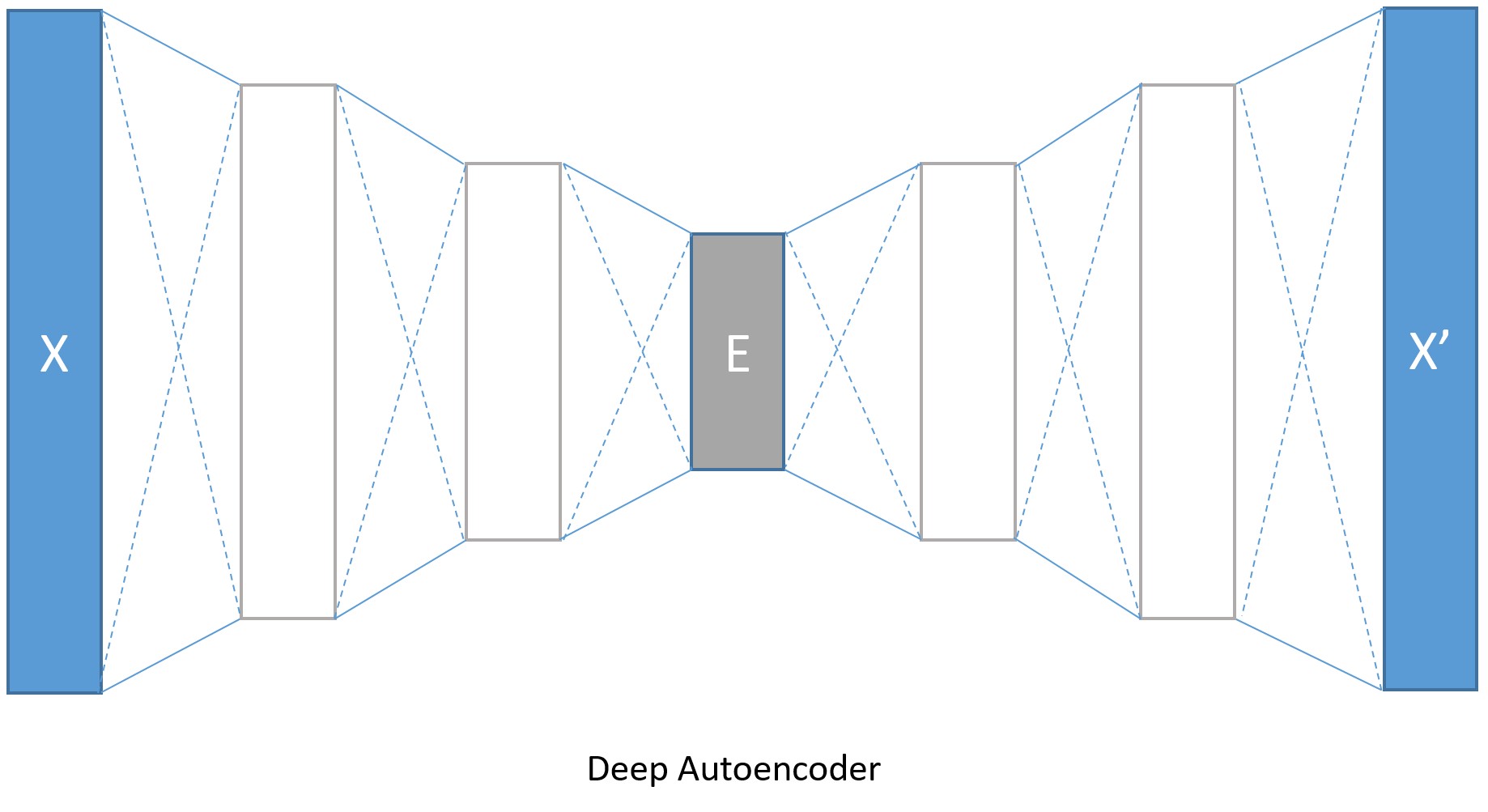
編碼層的大小分別是128,64,32,與之對應,解碼層就分別是64,128,784。轉換模型引數的增加會帶來更低的錯誤率,當然也會帶來訓練時間和記憶體佔用增多的代價。如果我們在訓練深度編碼器時將isFast設定成False,訓練就會進行更多輪,我們將得到更低的錯誤率,最後解碼的影象邊緣也會更清晰。
input_dim = 784
encoding_dims = [128,64,32]
decoding_dims = [64,128]

encoded_model = None

def create_deep_model(features):
    with C.layers.default_options(init = C.layers.glorot_uniform()):
        encode = C.element_times(C.constant(1.0/255.0), features)

        for encoding_dim in encoding_dims:
            encode = C.layers.Dense(encoding_dim, activation = C.relu)(encode)

        global encoded_model
        encoded_model= encode

        decode = encode
        for decoding_dim in decoding_dims:
            decode = C.layers.Dense(decoding_dim, activation = C.relu)(decode)

        decode = C.layers.Dense(input_dim, activation = C.sigmoid)(decode)
        return decode


num_label_classes = 10
reader_train = create_reader(train_file, True, input_dim, num_label_classes)
reader_test = create_reader(test_file, False, input_dim, num_label_classes)

model, deep_ae_train_error, deep_ae_test_error = train_and_test(reader_train, reader_test, model_func = create_deep_model)
結果:
 average      since    average      since      examples
    loss       last     metric       last
 ------------------------------------------------------
Learning rate per sample: 3e-05
      543        543      0.928      0.928            64
      543        543      0.925      0.923           192
      543        543      0.907      0.894           448
      542        541      0.891      0.877           960
      527        513      0.768      0.652          1984
      411        299       0.63      0.496          4032
      313        217      0.547      0.466          8128
      260        206      0.476      0.405         16320
      220        181      0.377      0.278         32704
      183        146      0.275      0.174         65472
      150        118      0.185     0.0947        131008
      125        100      0.119     0.0531        262080
Average training error: 10.90%
Average test error: 3.37%
視覺化深度自編碼器的結果
# Run the same image as the simple autoencoder through the deep encoder
orig_image = img_data[idx,:,:]
decoded_image = model.eval(orig_image)[0]*255

# Print image statistics
def print_image_stats(img, text):
    print(text)
    print("Max: {0:.2f}, Median: {1:.2f}, Mean: {2:.2f}, Min: {3:.2f}".format(np.max(img),np.median(img),np.mean(img),np.min(img)))

# Print original image
print_image_stats(orig_image, "Original image statistics:")

# Print decoded image
print_image_stats(decoded_image, "Decoded image statistics:")
然後我們把原始圖片和經過編碼解碼之後的圖片展示出來,理論上他們看起來應該挺像的
# Plot the original and the decoded image
img1 = orig_image.reshape(28,28)
text1 = 'Original image'

img2 = decoded_image.reshape(28,28)
text2 = 'Decoded image'

plot_image_pair(img1, text1, img2, text2)
我們上面展示了怎樣對一個輸入資料編碼和解碼。接下來我們會展示輸入資料之間的比較和如何從輸入資料中提取編碼之後的資料。t-SNE可能是將將高維資料視覺化成2D的最好方法,但是使用t-SNE時通常需要相對低維的資料,所以將資料使用自編碼器編碼成較低維度(比如32維)的資料,然後使用t-SNE對映成2D是一個比較好的方法。
所以接下來我們將使用深度自編碼器的輸出結果做如下工作:
- 壓縮/編碼兩個圖片
- 展示我們如何能得到兩個圖片編碼之後的資料。
首先我們需要讀取一些圖片和他們的標記
# Read some data to run get the image data and the corresponding labels
num_label_classes = 10
reader_viz = create_reader(test_file, False, input_dim, num_label_classes)

image = C.input_variable(input_dim)
image_label = C.input_variable(num_label_classes)

viz_minibatch_size = 50

viz_input_map = {
    image  : reader_viz.streams.features,
    image_label  : reader_viz.streams.labels_viz
}

viz_data = reader_eval.next_minibatch(viz_minibatch_size,
                                  input_map = viz_input_map)

img_data   = viz_data[image].asarray()
imglabel_raw = viz_data[image_label].asarray()


# Map the image labels into indices in minibatch array
img_labels = [np.argmax(imglabel_raw[i,:,:]) for i in range(0, imglabel_raw.shape[0])]

from collections import defaultdict
label_dict=defaultdict(list)
for img_idx, img_label, in enumerate(img_labels):
    label_dict[img_label].append(img_idx)

# Print indices corresponding to 3 digits
randIdx = [1, 3, 9]
for i in randIdx:
    print("{0}: {1}".format(i, label_dict[i]))
我們將使用scipy計算兩張圖片的餘弦距離。
from scipy import spatial

def image_pair_cosine_distance(img1, img2):
    if img1.size != img2.size:
        raise ValueError("Two images need to be of same dimension")
    return 1 - spatial.distance.cosine(img1, img2)


# Let s compute the distance between two images of the same number
digit_of_interest = 6

digit_index_list = label_dict[digit_of_interest]

if len(digit_index_list) < 2:
    print("Need at least two images to compare")
else:
    imgA = img_data[digit_index_list[0],:,:][0]
    imgB = img_data[digit_index_list[1],:,:][0]

    # Print distance between original image
    imgA_B_dist = image_pair_cosine_distance(imgA, imgB)
    print("Distance between two original image: {0:.3f}".format(imgA_B_dist))

    # Plot the two images
    img1 = imgA.reshape(28,28)
    text1 = 'Original image 1'

    img2 = imgB.reshape(28,28)
    text2 = 'Original image 2'

    plot_image_pair(img1, text1, img2, text2)

    # Decode the encoded stream
    imgA_decoded =  model.eval([imgA])[0]
    imgB_decoded =  model.eval([imgB])   [0]
    imgA_B_decoded_dist = image_pair_cosine_distance(imgA_decoded, imgB_decoded)

    # Print distance between original image
    print("Distance between two decoded image: {0:.3f}".format(imgA_B_decoded_dist))

    # Plot the two images
    # Plot the original and the decoded image
    img1 = imgA_decoded.reshape(28,28)
    text1 = 'Decoded image 1'

    img2 = imgB_decoded.reshape(28,28)
    text2 = 'Decoded image 2'

    plot_image_pair(img1, text1, img2, text2)
注:上餘弦距離如果是1表示兩個資料非常相似,餘弦距離是0表示一點都不相似。
任務2是如何獲取一個圖片編碼之後的向量資料。也就是要求在網路示意圖中標有E的部分。
imgA = img_data[digit_index_list[0],:,:][0]
imgA_encoded =  encoded_model.eval([imgA])

print("Length of the original image is {0:3d} and the encoded image is {1:3d}".format(len(imgA),len(imgA_encoded[0])))
print("\nThe encoded image: ")
print(imgA_encoded[0])
輸出:
Length of the original image is 784 and the encoded image is  32

The encoded image:
[  0.          22.22325325   3.9777317   13.26123905   9.97513866   0.
  13.37649727   6.18241978   5.78068304  12.50789165  20.11767769
   9.77285862   0.          14.75064278  17.07588768   0.           3.6076715
   8.29384613  20.11726952  15.80433846   3.4400022    0.           0.
  14.63469696   3.61723995  15.29668236  10.98176098   7.29611969
  16.65932465   9.66042233   5.93092394   0.        ]
我們來比較一下不同數字之間的餘弦距離
digitA = 3
digitB = 8

digitA_index = label_dict[digitA]
digitB_index = label_dict[digitB]

imgA = img_data[digitA_index[0],:,:][0]
imgB = img_data[digitB_index[0],:,:][0]

# Print distance between original image
imgA_B_dist = image_pair_cosine_distance(imgA, imgB)
print("Distance between two original image: {0:.3f}".format(imgA_B_dist))

# Plot the two images
img1 = imgA.reshape(28,28)
text1 = 'Original image 1'

img2 = imgB.reshape(28,28)
text2 = 'Original image 2'

plot_image_pair(img1, text1, img2, text2)

# Decode the encoded stream
imgA_decoded =  model.eval([imgA])[0]
imgB_decoded =  model.eval([imgB])[0]
imgA_B_decoded_dist = image_pair_cosine_distance(imgA_decoded, imgB_decoded)

#Print distance between original image
print("Distance between two decoded image: {0:.3f}".format(imgA_B_decoded_dist))

# Plot the original and the decoded image
img1 = imgA_decoded.reshape(28,28)
text1 = 'Decoded image 1'

img2 = imgB_decoded.reshape(28,28)
text2 = 'Decoded image 2'

plot_image_pair(img1, text1, img2, text2)
歡迎掃碼關注我的微信公眾號獲取最新文章
