
Python資料分析基礎教程:Numpy學習指南
第二章 Numpy基礎
2.6 改變陣列維度
ravel()、flatten() 將多維陣列展平
b.transpose() 矩陣轉置,等同於b.T,一維陣列不變
reshape() 改變陣列維度
2.8 組合陣列
hstack((a, b)) 水平組合,等同於 concatenate((a, b), axis=1)
vstack((a, b)) 垂直組合,等同於 concatenate((a, b), axis=0)
column_stack((a, b)) 列組合,二維等同於hstack
row_stack((a, b)) 行組合,二維等同與vstack
2.10 分割陣列
In: a
Out:
array([[0 vsplit(a,3) 垂直分割 ,等同於 split(a,3,axis=0)
2.11 陣列屬性
ndim 陣列維度,或陣列軸的個數
size 陣列元素總數
itemsize 陣列元素在記憶體中所佔位元組數
nbytes 陣列所佔儲存空間 = itemsize * size
b = array([1.j + 1, 2.j + 3]) 虛數
b.real 複數陣列的實部 b.imag 虛部
flat屬性將返回一個numpy.flatiter物件,可以讓我們像遍歷一維陣列一樣去遍歷任意的多維陣列。
In: b = arange(4).reshape(2,2)
In: b
Out:
array([[0, 1],
[2, 3]])
In: f = b.flat
In: f
Out: <numpy.flatiter object at 0x103013e00>
In: for item in f: print 2.12 陣列轉換
tolist函式將NumPy陣列轉換成Python列表。
In: b
Out: array([ 1.+1.j, 3.+2.j])
In: b.tolist()
Out: [(1+1j), (3+2j)]
astype函式可以在轉換陣列時指定資料型別。
In: b
Out: array([ 1.+1.j, 3.+2.j])
In: b.astype(int)
/usr/local/bin/ipython:1: ComplexWarning: Casting complex values to real discards the imaginary part #虛部丟失,轉為b.astype('complex') 則不會發生錯誤。

#!/usr/bin/python
Out: array([1, 3])
3.2 讀寫檔案
savetxt
import numpy as np
i2 = np.eye(2)
np.savetxt("eye.txt", i2)
3.4 讀入CSV檔案
# AAPL,28-01-2011, ,344.17,344.4,333.53,336.1,21144800

c,v=np.loadtxt('data.csv', delimiter=',', usecols=(6,7), unpack=True) #index從0開始
3.6.1 算術平均值
np.mean(c) = np.average(c)
3.6.2 加權平均值
t = np.arange(len(c))
np.average(c, weights=t)
3.8 極值
np.min(c)
np.max(c)
np.ptp(c) 最大值與最小值的差值
3.10 統計分析
np.median(c) 中位數
np.msort(c) 升序排序
np.var(c) 方差
3.12 分析股票收益率
np.diff(c) 可以返回一個由相鄰陣列元素的差
值構成的陣列
returns = np.diff( arr ) / arr[ : -1] #diff返回的陣列比收盤價陣列少一個元素np.std(c) 標準差
對數收益率
logreturns = np.diff( np.log(c) ) #應檢查輸入陣列以確保其不含有零和負數where 可以根據指定的條件返回所有滿足條件的數
組元素的索引值。
posretindices = np.where(returns > 0)
np.sqrt(1./252.) 平方根,浮點數
3.14 分析日期資料
# AAPL,28-01-2011, ,344.17,344.4,333.53,336.1,21144800

dates, close=np.loadtxt('data.csv', delimiter=',', usecols=(1,6), converters={1:datestr2num}, unpack=True)
print "Dates =", dates

def datestr2num(s):
    return datetime.datetime.strptime(s, "%d-%m-%Y").date().weekday()
# 星期一 0
# 星期二 1
# 星期三 2
# 星期四 3
# 星期五 4
# 星期六 5
# 星期日 6

#output
Dates = [ 4. 0. 1. 2. 3. 4. 0. 1. 2. 3. 4. 0. 1. 2. 3. 4. 1. 2. 4. 0. 1. 2. 3. 4. 0.
1. 2. 3. 4.]
averages = np.zeros(5)
for i in range(5):
indices = np.where(dates == i)
prices = np.take(close, indices) #按陣列的元素運算,產生一個數組作為輸出。
>>> a = [4, 3, 5, 7, 6, 8]
>>> indices = [0, 1, 4]
>>> np.take(a, indices)
array([4, 3, 6])np.argmax(c) #返回的是陣列中最大元素的索引值
np.argmin(c)
3.16 彙總資料
# AAPL,28-01-2011, ,344.17,344.4,333.53,336.1,21144800

#得到第一個星期一和最後一個星期五
first_monday = np.ravel(np.where(dates == 0))[0]
last_friday = np.ravel(np.where(dates == 4))[-1]

#建立一個數組,用於儲存三週內每一天的索引值
weeks_indices = np.arange(first_monday, last_friday + 1)
#按照每個子陣列5個元素,用split函式切分陣列
weeks_indices = np.split(weeks_indices, 5)
#output
[array([1, 2, 3, 4, 5]), array([ 6, 7, 8, 9, 10]), array([11,12, 13, 14, 15])]

weeksummary = np.apply_along_axis(summarize, 1, weeks_indices,open, high, low, close)

def summarize(a, o, h, l, c): #open, high, low, close
monday_open = o[a[0]]
week_high = np.max( np.take(h, a) )
week_low = np.min( np.take(l, a) )
friday_close = c[a[-1]]
return("APPL", monday_open, week_high, week_low, friday_close)

np.savetxt("weeksummary.csv", weeksummary, delimiter=",", fmt="%s") #指定了檔名、需要儲存的陣列名、分隔符(在這個例子中為英文標點逗號)以及儲存浮點數的格式。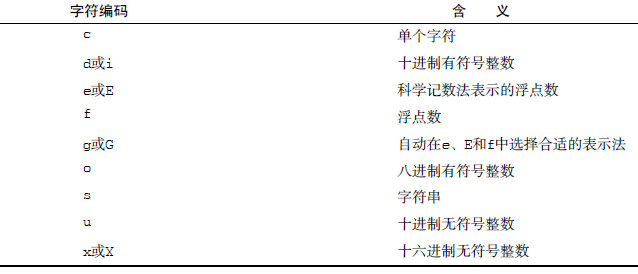
格式字串以一個百分號開始。接下來是一個可選的標誌字元:-表示結果左對齊,0表示左端補0,+表示輸出符號(正號+或負號-)。第三部分為可選的輸出寬度引數,表示輸出的最小位數。第四部分是精度格式符,以”.”開頭,後面跟一個表示精度的整數。最後是一個型別指定字元,在例子中指定為字串型別。
numpy.apply_along_axis(func1d, axis, arr, *args, **kwargs)
>>> def my_func(a):
...     """Average first and last element of a 1-D array"""
...     return (a[0] + a[-1]) * 0.5
>>> b = np.array([[1,2,3], [4,5,6], [7,8,9]])
>>> np.apply_along_axis(my_func, 0, b)  #沿著X軸運動,取列切片
array([ 4.,  5.,  6.])
>>> np.apply_along_axis(my_func, 1, b)  #沿著y軸運動,取行切片
array([ 2.,  5.,  8.])


>>> b = np.array([[8,1,7], [4,3,9], [5,2,6]])
>>> np.apply_along_axis(sorted, 1, b)
array([[1, 7, 8],
       [3, 4, 9],
       [2, 5, 6]])
3.20 計算簡單移動平均線
(1) 使用ones函式建立一個長度為N的元素均初始化為1的陣列,然後對整個陣列除以N,即可得到權重。如下所示:
N = int(sys.argv[1])
weights = np.ones(N) / N
print "Weights", weights
在N = 5時,輸出結果如下:
Weights [ 0.2 0.2 0.2 0.2 0.2] #權重相等(2) 使用這些權重值,呼叫convolve函式:
c = np.loadtxt('data.csv', delimiter=',', usecols=(6,),unpack=True)
sma = np.convolve(weights, c)[N-1:-N+1]   #卷積是分析數學中一種重要的運算,定義為一個函式與經過翻轉和平移的另一個函式的乘積的積分。

t = np.arange(N - 1, len(c))   #作圖
plot(t, c[N-1:], lw=1.0)
plot(t, sma, lw=2.0)
show()
3.22 計算指數移動平均線
指數移動平均線(exponential moving average)。指數移動平均線使用的權重是指數衰減的。對歷史上的資料點賦予的權重以指數速度減小,但永遠不會到達0。
x = np.arange(5)
print "Exp", np.exp(x)
#output
Exp [ 1. 2.71828183 7.3890561 20.08553692 54.59815003]
Linspace 返回一個元素值在指定的範圍內均勻分佈的陣列。
print "Linspace", np.linspace(-1, 0, 5) #起始值、終止值、可選的元素個數
#output
Linspace [-1. -0.75 -0.5 -0.25 0. ]
(1)權重計算
N = int(sys.argv[1])
weights = np.exp(np.linspace(-1. , 0. , N))
(2)權重歸一化處理
weights /= weights.sum()
print "Weights", weights
#output
Weights [ 0.11405072 0.14644403 0.18803785 0.24144538 0.31002201]
(3)計算及作圖
c = np.loadtxt('data.csv', delimiter=',', usecols=(6,),unpack=True)
ema = np.convolve(weights, c)[N-1:-N+1]
t = np.arange(N - 1, len(c))
plot(t, c[N-1:], lw=1.0)
plot(t, ema, lw=2.0)
show()
3.26 用線性模型預測價格
(x, residuals, rank, s) = np.linalg.lstsq(A, b) #係數向量x、一個殘差陣列、A的秩以及A的奇異值
print x, residuals, rank, s
#計算下一個預測值
print np.dot(b, x)
3.28 繪製趨勢線
>>> x = np.arange(6)
>>> x = x.reshape((2, 3))
>>> x
array([[0, 1, 2],
       [3, 4, 5]])
>>> np.ones_like(x)   #用1填充陣列
array([[1, 1, 1],
       [1, 1, 1]])
類似函式
zeros_like
empty_like
zeros
ones
empty
3.30 陣列的修剪和壓縮
a = np.arange(5)
print "a =", a
print "Clipped", a.clip(1, 2) #將所有比給定最大值還大的元素全部設為給定的最大值,而所有比給定最小值還小的元素全部設為給定的最小值
#output
a = [0 1 2 3 4]
Clipped [1 1 2 2 2]
a = np.arange(4)
print a
print "Compressed", a.compress(a > 2) #返回一個根據給定條件篩選後的陣列
#output
[0 1 2 3]
Compressed [3]b = np.arange(1, 9)
print "b =", b
print "Factorial", b.prod() #輸出陣列元素階乘結果
#output
b = [1 2 3 4 5 6 7 8]
Factorial 40320
print "Factorials", b.cumprod()
#output
Factorials [ 1 2 6 24 120 720 5040 40320] #陣列元素遍歷階乘4.2 股票相關性分析
covariance = np.cov(a,b)
獲取對角元素
covariance.diagonal()
4.4 多項式擬合
bhp=np.loadtxt('BHP.csv', delimiter=',', usecols=(6,), unpack=True)
vale=np.loadtxt('VALE.csv', delimiter=',', usecols=(6,),unpack=True)
t = np.arange(len(bhp))
poly = np.polyfit(t, bhp - vale, int(sys.argv[1])) # sys.argv[1]為3,即用3階多項式擬合數據
print "Polynomial fit", poly

#output
Polynomial fit [ 1.11655581e-03 -5.28581762e-02 5.80684638e-01 5.79791202e+01]
#預測下個值
print "Next value", np.polyval(poly, t[-1] + 1)
使用polyder函式對多項式函式求導(以求極值)
der = np.polyder(poly)
print "Derivative", der
#output
Derivative [ 0.00334967 -0.10571635 0.58068464]
求出導數函式的根,即找出原多項式函式的極值點
print "Extremas", np.roots(der)
#output
Extremas [ 24.47820054 7.08205278]
注:書中提示,3階多項式擬合數據的結果並不好,可嘗試更高階的多項式擬合。
4.6 計算OBV(On-Balance Volume)淨額成交量
diff函式可以計算陣列中兩個連續元素的差值,並返回一個由這些差值組成的陣列。
change = np.diff(c)
sign函式可以返回陣列中每個元素的正負符號,陣列元素為負時返回-1,為正時返回1,否則返回0
np.sign(change)
使用piecewise(分段的)函式來獲取陣列元素的正負。使用合適的返回值和對應的條件呼叫該函式:
pieces = np.piecewise(change, [change < 0, change > 0], [-1, 1])
print "Pieces", pieces
檢查一致性
np.array_equal(a, b)
np.vectorize 替代迴圈
>>> def myfunc(a, b):
...     "Return a-b if a>b, otherwise return a+b"
...     if a > b:
...         return a - b
...     else:
...         return a + b

>>> vfunc = np.vectorize(myfunc)
>>> vfunc([1, 2, 3, 4], 2)
array([3, 4, 1, 2])
The vectorize function is provided primarily for convenience, not for performance. The implementation is essentially a for loop.
4.10 使用hanning 函式平滑資料
(1) 呼叫hanning函式計算權重,生成一個長度為N的視窗(在這個示例中N取8)
N = int(sys.argv[1])
weights = np.hanning(N)
print "Weights", weights

#output
Weights [ 0. 0.1882551 0.61126047 0.95048443 0.95048443 0.61126047 0.1882551 0. ]

bhp = np.loadtxt('BHP.csv', delimiter=',', usecols=(6,),unpack=True)   #某股票資料
bhp_returns = np.diff(bhp) / bhp[ : -1] #股票收益率計算
smooth_bhp = np.convolve(weights/weights.sum(), bhp_returns) [N-1:-N+1]  #使用weights平滑股票收益率

#繪圖
t = np.arange(N - 1, len(bhp_returns))
plot(t, bhp_returns[N-1:], lw=1.0)
plot(t, smooth_bhp, lw=2.0)
show()
兩個多項式做差運算
poly_sub = np.polysub(a, b)
選擇函式
numpy.select(condlist, choicelist, default=0)
>>> x = np.arange(10)
>>> condlist = [x<3, x>5]
#輸出兩個array [true...false...],[false,...true]
>>> choicelist = [x, x**2]
>>> np.select(condlist, choicelist)
array([ 0,  1,  2,  0,  0,  0, 36, 49, 64, 81])
trim_zeros函式可以去掉一維陣列中開頭和末尾為0的元素:
np.trim_zeros(a)
5.2 建立矩陣(略)
5.4 從已有矩陣建立新矩陣(略)
5.6 建立通用函式(略)
5.7 通用函式的方法(略)
5.8 在add上呼叫通用函式的方法(略)
5.10 陣列的除法運算
在NumPy中,基本算術運算子+、-和*隱式關聯著通用函式add、subtract和multiply。
也就是說,當你對NumPy陣列使用這些算術運算子時,對應的通用函式將自動被呼叫。除法包含的過程則較為複雜,在陣列的除法運算中涉及三個通用函式divide、true_divide和floor_division,以及兩個對應的運算子/和//。
a = np.array([2, 6, 5])
b = np.array([1, 2, 3])
print "Divide", np.divide(a, b), np.divide(b, a)
#output
Divide [2 3 1] [0 0 0]

print "True Divide", np.true_divide(a, b), np.true_divide(b, a)
#output
True Divide [2. 3. 1.66666667] [0.5 0.33333333 0.6 ]


print "Floor Divide", np.floor_divide(a, b), np.floor_divide(b, a) c = 3.14 * b   #floor_divide函式總是返回整數結果,相當於先呼叫divide函式再呼叫floor函式。
print "Floor Divide 2", np.floor_divide(c, b), np.floor_divide(b, c) #floor函式將對浮點數進行向下取整並返回整數。

#output
Floor Divide [2 3 1] [0 0 0]
Floor Divide 2 [ 3. 3. 3.] [ 0. 0. 0.]
預設情況下,使用/運算子相當於呼叫divide函式
運算子//對應於floor_divide函式
print "// operator", a//b, b//a5.12 模運算
remainder函式逐個返回兩個陣列中元素相除後的餘數。如果第二個數字為0,則直接返回0。
a = np.arange(-4, 4)
print "Remainder", np.remainder(a, 2) #等同於a % 2
#output
Remainder [0 1 0 1 0 1 0 1]
mod函式與remainder函式的功能完全一致
fmod函式處理負數的方式與remainder、mod和%不同。所得餘數的正負由被除數決定,與除數的正負無關。
print "Fmod", np.fmod(a, 2)
#output
Fmod [ 0 -1 0 -1 0 1 0 1]
5.14 計算斐波那契數列
rint函式對浮點數取整,但結果仍為浮點數型別
a = np.arange(1,3,0.5) #[1.,1.5,2.,2.5]
pr int np.rint(a) #[1.,2.,2.,2.]5.18 繪製方波(略)
5.20 繪製鋸齒波和三角波(略)
5.22 玩轉二進位制位
三個運用位操作的小技巧——檢查兩個整數的符號是否一致,檢查一個數是否為2的冪數,以及計算一個數被2的冪數整除後的餘數。
XOR或者^操作符。XOR操作符又被稱為不等運算子,因此當兩個運算元的符號不一致時,XOR操作的結果為負數。
import numpy as np
x = np.arange(-9, 9)
y = -x
print "Sign different?", (x ^ y) < 0
print "Sign different?", np.less(np.bitwise_xor(x, y), 0) #^操作符對應於bitwise_xor函式,<操作符對應於less函式
在二進位制數中,2的冪數表示為一個1後面跟一串0的形式,例如10、100、1000等。而比2的冪數小1的數表示為一串二進位制的1,例如11、111、1111(即十進位制裡的3、7、15)等。如果我們在2的冪數以及比它小1的數之間執行位與操作AND,那麼應該得到0。
print "Power of 2?\n", x, "\n", (x & (x - 1)) == 0
print "Power of 2?\n", x, "\n", np.equal(np.bitwise_and(x, (x - 1)), 0) #&操作符對應於bitwise_and函式,==操作符對應於equal函式。
計算餘數的技巧實際上只在模為2的冪數(如4、8、16等)時有效。二進位制的位左移一位,則數值翻倍。在前一個小技巧中我們看到,將2的冪數減去1可以得到一串1組成的二進位制數,如11、111、1111等。這為我們提供了掩碼(mask),與這樣的掩碼做位與操作AND即可得到以2的冪數作為模的餘數。
print "Modulus 4\n", x, "\n", x & ((1 << 2) - 1)
print "Modulus 4\n", x, "\n", np.bitwise_and(x, np.left_shift(1, 2) - 1) #<<操作符對應於left_shift函式
6.2 計算逆矩陣(略)
6.3 求解線性方程
A = np.mat("1 -2 1;0 2 -8;-4 5 9")
b = np.array([0, 8, -9])
x = np.linalg.solve(A, b)
6.6 求解特徵值和特徵向量(略)
6.8 分解矩陣(略)
6.10 計算廣義逆矩陣(略)
6.12 計算矩陣的行列式(略)
6.14 計算傅立葉變換(略)
6.16 移頻(略)
6.18 硬幣賭博遊戲
對一個硬幣賭博遊戲下8份賭注。每一輪拋9枚硬幣,如果少於5枚硬幣正面朝上,將損失8份賭注中的1份;否則,將贏得1份賭注。模擬一下賭博的過程,初始資本為1000份賭注。
import numpy as np
from matplotlib.pyplot import plot, show
cash = np.zeros(10000) #將在賭場中玩10000輪硬幣賭博遊戲。
cash[0] = 1000
outcome = np.random.binomial(9, 0.5, size=len(cash)) #二項式分佈
for i in range(1, len(cash)):
    if outcome[i] < 5:
        cash[i] = cash[i - 1] - 1
    elif outcome[i] < 10:
        cash[i] = cash[i - 1] + 1
    else:
        raise AssertionError("Unexpected outcome " + outcome)

print outcome.min(), outcome.max()
plot(np.arange(len(cash)), cash)
show() #剩餘資本呈隨機遊走(random walk)狀態
6.20 模擬遊戲秀節目
超幾何分佈(hypergeometric distribution)是一種離散概率分佈,它描述的是一個罐子裡有兩種物件,無放回地從中抽取指定數量的物件後,抽出指定種類物件的數量。
設想有這樣一個遊戲秀節目,每當參賽者回答對一個問題,他們可以從一個罐子裡摸出3個球並放回。罐子裡有一個“倒黴球”,一旦這個球被摸出,參賽者會被扣去6分。而如果他們摸出的3個球全部來自其餘的25個普通球,那麼可以得到1分。因此,如果一共有100道問題被正確回答,得分情況會是怎樣的呢?
(1) 使用hypergeometric函式初始化遊戲的結果矩陣。該函式的第一個引數為罐中普通球的數量,第二個引數為“倒黴球”的數量,第三個引數為每次取樣(摸球)的數量。
points = np.zeros(100)
outcomes = np.random.hypergeometric(25, 1, 3, size=len(points))
(2) 根據上一步產生的遊戲結果計算相應的得分。
for i in range(len(points)):
    if outcomes[i] == 3:
        points[i] = points[i - 1] + 1
    elif outcomes[i] == 2:
        points[i] = points[i - 1] - 6
    else:
        print outcomes[i]
(3) 使用Matplotlib繪製points陣列。
plot(np.arange(len(points)), points)
show()
6.22 正態分佈
連續分佈可以用PDF(Probability Density Function,概率密度函式)來描述。隨機變數落在某一區間內的概率等於概率密度函式在該區間的曲線下方的面積。
(1) 使用NumPy random模組中的normal函式產生指定數量的隨機數。
N=10000
normal_values = np.random.normal(size=N)(2) 繪製分佈直方圖和理論上的概率密度函式(均值為0、方差為1的正態分佈)曲線。使用Matplotlib進行繪圖。
dummy, bins, dummy = plt.hist(normal_values, np.sqrt(N), normed=True, lw=1)
sigma = 1
mu = 0
plt.plot(bins, 1/(sigma * np.sqrt(2 * np.pi)) * np.exp( - (bins -mu)**2 / (2 *sigma**2) ),lw=2)
plt.show()
6.24 對數正態分佈
對數正態分佈(lognormal distribution) 是自然對數服從正態分佈的任意隨機變數的概率分佈。
(1) 使用NumPy random模組中的normal函式產生隨機數。
N=10000
lognormal_values = np.random.lognormal(size=N)
(2) 繪製分佈直方圖和理論上的概率密度函式(均值為0、方差為1)。我們將使用Matplotlib進行繪圖。
dummy, bins, dummy = plt.hist(lognormal_values,np.sqrt(N), normed=True, lw=1)
sigma = 1
mu = 0
x = np.linspace(min(bins), max(bins), len(bins))
pdf = np.exp(-(numpy.log(x) - mu)**2 / (2 * sigma**2))/ (x *sigma * np.sqrt(2 * np.pi))
plt.plot(x, pdf,lw=3)
plt.show()
7.1 排序
NumPy提供了多種排序函式,如下所示:
sort函式返回排序後的陣列;
lexsort函式根據鍵值的字典序進行排序;
argsort函式返回輸入陣列排序後的下標;
ndarray類的sort方法可對陣列進行原地排序;
msort函式沿著第一個軸排序;
sort_complex函式對複數按照先實部後虛部的順序進行排序。
7.2 按字典序排序
lexsort函式返回輸入陣列按字典序排序後的下標
Sort names: first by surname, then by name.
>>> surnames =    ('Hertz',    'Galilei', 'Hertz')
>>> first_names = ('Heinrich', 'Galileo', 'Gustav')
>>> ind = np.lexsort((first_names, surnames))
>>> ind
array([1, 2, 0])
>>>
>>> [surnames[i] + ", " + first_names[i] for i in ind]
['Galilei, Galileo', 'Hertz, Gustav', 'Hertz, Heinrich']
Sort two columns of numbers:
>>> a = [1,5,1,4,3,4,4] # First column
>>> b = [9,4,0,4,0,2,1] # Second column
>>> ind = np.lexsort((b,a)) # Sort by a, then by b
>>> print ind
[2 0 4 6 5 3 1]
>>>
>>> [(a[i],b[i]) for i in ind]
[(1, 0), (1, 9), (3, 0), (4, 1), (4, 2), (4, 4), (5, 4)]
7.4 對複數進行排序(略)
7.5 搜尋
argmax函式返回陣列中最大值對應的下標。
>>> a = np.array([2, 4, 8])
>>> np.argmax(a)
2 nanargmax函式提供相同的功能,但忽略NaN值。
>>> b = np.array([np.nan, 2, 4])
>>> np.nanargmax(b)
2 argmin和nanargmin函式的功能類似,只不過換成了最小值。
argwhere函式根據條件搜尋非零的元素,並分組返回對應的下標。
>>> a = np.array([2, 4, 8])
>>> np.argwhere(a <= 4)
array([[0],[1]]) searchsorted函式可以為指定的插入值尋找維持陣列排序的索引位置。該函式使用二分搜尋演算法,計算複雜度為O(log(n))。
extract函式返回滿足指定條件的陣列元素。
7.6 使用searchsorted 函式
searchsorted函式為7和-2返回了索引5和0。用這些索引作為插入位置,生成陣列[-2, 0, 1, 2, 3, 4, 7],這樣就維持了陣列的排序
import numpy as np
a = np.arange(5)
indices = np.searchsorted(a, [-2, 7])  #索引可以維持陣列排序的插入位置
print "Indices", indices
#output
Indices [0 5]

print "The full array", np.insert(a, indices, [-2, 7])
#output
The full array [-2 0 1 2 3 4 7]
7.8 從陣列中抽取元素
從一個數組中抽取偶數元素。
import numpy as np
a = np.arange(7)
condition = (a % 2) == 0 #生成選擇偶數元素的條件變數
print "Even numbers", np.extract(condition, a)
print "Non zero", np.nonzero(a)
使用nonzero函式抽取陣列中的非零元素
np.nonzero(a)
7.9 金融函式
fv函式計算所謂的終值(future value),即基於一些假設給出的某個金融資產在未來某一時間點的價值。
pv函式計算現值(present value),即金融資產當前的價值。
npv函式返回的是淨現值(net present value),即按折現率計算的淨現金流之和。
pmt函式根據本金和利率計算每期需支付的金額。
irr函式計算內部收益率(internal rate of return)。內部收益率是是淨現值為0時的有效利率,不考慮通脹因素。
mirr函式計算修正後內部收益率(modified internal rate of return),是內部收益率的改進版本。
nper函式計算定期付款的期數。
rate函式計算利率(rate of interest)。
7.10 計算終值
終值是基於一些假設給出的某個金融資產在未來某一時間點的價值。終值決定於4個引數——利率、期數、每期支付金額以及現值。在本節的教程中,我們以利率3%、每季度支付金額10、存款週期5年以及現值1 000為引數計算終值。
使用正確的引數呼叫fv函式,計算終值:
print "Future value", np.fv(0.03/4, 5 * 4, -10, -1000)
#output
Future value 1376.09633204
7.12 計算現值(略)
7.14 計算淨現值(略)
7.16 計算內部收益率(略)
7.18 計算分期付款
pmt函式可以根據利率和期數計算貸款每期所需支付的資金。
假設貸款100萬,年利率為10%,要用30年時間還完貸款,那麼每月必須支付多少資金呢?使用剛才提到的引數值,呼叫pmt函式。
print "Payment", np.pmt(0.10/12, 12 * 30, 1000000)
#output
Payment -8775.71570089
7.20 計算付款期數
NumPy中的nper函式可以計算分期付款所需的期數。所需的引數為貸款利率、固定的月供以及貸款額。
考慮貸款9000,年利率10%,每月固定還款為100的情形。
通過nper函式計算出付款期數。
print "Number of payments", np.nper(0.10/12, -100, 9000)
#output
Number of payments 167.047511801 #需要167個月
7.22 計算利率
rate函式根據給定的付款期數、每期付款資金、現值和終值計算利率。
使用7.20節中的數值進行逆向計算,由其他引數得出利率。
填入之前教程中的數值作為引數。
print "Interest rate", 12 * np.rate(167, -100, 9000, 0)
#計算出的利率約為10%。
Interest rate 0.0999756420664
7.23 窗函式
窗函式(window function)是訊號處理領域常用的數學函式,相關應用包括譜分析和濾波器設計等。這些窗函式除在給定區間之外取值均為0。NumPy中有很多窗函式,如bartlett、blackman、hamming、hanning和kaiser。
7.24 繪製巴特利特窗
巴特利特窗(Bartlett window)是一種三角形平滑窗。
window = np.bartlett(42)
plot(window)
show()
7.25 布萊克曼窗
布萊克曼窗(Blackman window)形式上為三項餘弦值的加和。blackman函式返回布萊克曼窗。該函式唯一的引數為輸出點的數量。如果數量為0或小於0,則返回一個空陣列。
7.26 使用布萊克曼窗平滑股價資料(略)
7.27 漢明窗
漢明窗(Hamming window)形式上是一個加權的餘弦函式。NumPy中的hamming函式返回漢明窗。該函式唯一的引數為輸出點的數量。如果數量為0或小於0,則返回一個空陣列。
7.28 繪製漢明窗
window = np.hamming(42)
plot(window)
show()
7.29 凱澤窗
凱澤窗(Kaiser window)是以貝塞爾函式(Bessel function)定義的,該函式的第一個數為輸出點的數量。如果數量為0或小於0,則返回一個空陣列。第二個引數為β值。
window = np.kaiser(42, 14)
plot(window)
show()
7.31 專用數學函式(略)
7.32 繪製修正的貝塞爾函式(略)
7.34 繪製sinc 函式(略)
8.1 斷言函式
numpy.testing包:
- assert_almost_equal 如果兩個數字的近似程度沒有達到指定精度,就丟擲異常
- assert_approx_equal 如果兩個數字的近似程度沒有達到指定有效數字,就丟擲異常
- assert_array_almost_equal 如果兩個陣列中元素的近似程度沒有達到指定精度,就丟擲異常
- assert_array_equal 如果兩個陣列物件不相同,就丟擲異常
- assert_array_less 兩個陣列必須形狀一致,並且第一個陣列的元素嚴格小於第二個陣列的元素,否則就丟擲異常
- assert_equal 如果兩個物件不相同,就丟擲異常
- assert_raises 若用填寫的引數呼叫函式沒有丟擲指定的異常,則測試不通過
- assert_warns 若沒有丟擲指定的警告,則測試不通過
- assert_string_equal 斷言兩個字串變數完全相同
- assert_allclose 如果兩個物件的近似程度超出了指定的容差限,就丟擲異常
8.2 使用assert_almost_equal 斷言近似相等
(1) 呼叫函式,指定較低的精度(小數點後7位):
print "Decimal 6", np.testing.assert_almost_equal(0.123456789, 0.123456780,decimal=7)
#output
Decimal 6 None
(2) 呼叫函式,指定較高的精度(小數點後8位):
print "Decimal 7", np.testing.assert_almost_equal(0.123456789, 0.123456780,decimal=8)

#output
Decimal 7
Traceback (most recent call last):
...
raiseAssertionError(msg)
AssertionError:
Arrays are not almost equal
ACTUAL: 0.123456789
DESIRED: 0.12345678
8.4 使用assert_approx_equal 斷言近似相等
與assert_almost_equal 類似,以小數點後7位為分界點。
8.6 斷言陣列近似相等
assert_array_almost_equal函式將丟擲異常。該函式首先檢查兩個陣列的形狀是否一致,然後逐一