吳恩達deeplearning.ai課程作業，自己寫的答案。
補充說明：
1. 評論中總有人問為什麼直接複製這些notebook執行不了？請不要直接複製貼上，不可能執行通過的，這個只是notebook中我們要自己寫的那部分，要正確執行還需要其他py檔案，請自己到GitHub上下載完整的。這裡的部分僅僅是參考用的，建議還是自己按照提示一點一點寫，如果實在卡住了再看答案。個人覺得這樣才是正確的學習方法，況且作業也不算難。
2. 關於評論中有人說我是抄襲，註釋還沒別人詳細，複製下來還執行不過。答覆是：做伸手黨之前，請先搞清這個作業是幹什麼的。大家都是從GitHub上下載原始的作業，然後根據程式碼前面的提示（通常會指定函式和公式）來編寫程式碼，而且後面還有expected output供你比對，如果程式正確，結果一般來說是一樣的。請不要無腦噴，說什麼跟別人的答案一樣的。說到底，我們要做的就是，看他的文字部分，根據提示在程式碼中加入部分自己的程式碼。我們自己要寫的部分只有那麼一小部分程式碼。
3. 由於實在很反感無腦噴子，故禁止了下面的評論功能，請見諒。如果有問題，請私信我，在力所能及的範圍內會盡量幫忙。

Deep Neural Network for Image Classification: Application

When you finish this, you will have finished the last programming assignment of Week 4, and also the last programming assignment of this course!

You will use use the functions you’d implemented in the previous assignment to build a deep network, and apply it to cat vs non-cat classification. Hopefully, you will see an improvement in accuracy relative to your previous logistic regression implementation.

After this assignment you will be able to:
- Build and apply a deep neural network to supervised learning.

Let’s get started!

1 - Packages

Let’s first import all the packages that you will need during this assignment.
- numpy is the fundamental package for scientific computing with Python.
-

matplotlib is a library to plot graphs in Python.
- h5py is a common package to interact with a dataset that is stored on an H5 file.
- PIL and scipy are used here to test your model with your own picture at the end.
- dnn_app_utils provides the functions implemented in the “Building your Deep Neural Network: Step by Step” assignment to this notebook.
- np.random.seed(1) is used to keep all the random function calls consistent. It will help us grade your work.

import time
import numpy as np
import h5py
import matplotlib.pyplot as plt
import scipy
from PIL import Image
from scipy import ndimage
from dnn_app_utils_v2 import *

%matplotlib inline
plt.rcParams['figure.figsize'] = (5.0, 4.0) # set default size of plots
plt.rcParams['image.interpolation'] = 'nearest'
plt.rcParams['image.cmap'] = 'gray'

%load_ext autoreload
%autoreload 2

np.random.seed(1)

2 - Dataset

You will use the same “Cat vs non-Cat” dataset as in “Logistic Regression as a Neural Network” (Assignment 2). The model you had built had 70% test accuracy on classifying cats vs non-cats images. Hopefully, your new model will perform a better!

Problem Statement: You are given a dataset (“data.h5”) containing:
- a training set of m_train images labelled as cat (1) or non-cat (0)
- a test set of m_test images labelled as cat and non-cat
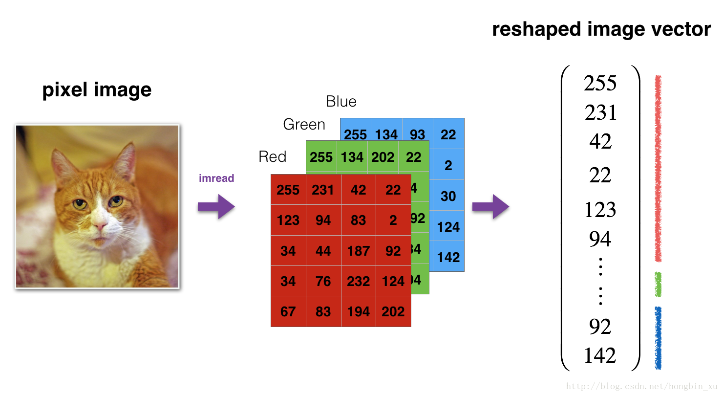
- each image is of shape (num_px, num_px, 3) where 3 is for the 3 channels (RGB).

Let’s get more familiar with the dataset. Load the data by running the cell below.

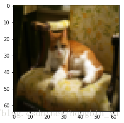
train_x_orig, train_y, test_x_orig, test_y, classes = load_data()

The following code will show you an image in the dataset. Feel free to change the index and re-run the cell multiple times to see other images.

# Example of a picture
index = 7
plt.imshow(train_x_orig[index])
print ("y = " + str(train_y[0,index]) + ". It's a " + classes[train_y[0,index]].decode("utf-8") +  " picture.")

y = 1. It's a cat picture.

# Explore your dataset 
m_train = train_x_orig.shape[0]
num_px = train_x_orig.shape[1]
m_test = test_x_orig.shape[0]

print ("Number of training examples: " + str(m_train))
print ("Number of testing examples: " + str(m_test))
print ("Each image is of size: (" + str(num_px) + ", " + str(num_px) + ", 3)")
print ("train_x_orig shape: " + str(train_x_orig.shape))
print ("train_y shape: " + str(train_y.shape))
print ("test_x_orig shape: " + str(test_x_orig.shape))
print ("test_y shape: " + str(test_y.shape))

Number of training examples: 209
Number of testing examples: 50
Each image is of size: (64, 64, 3)
train_x_orig shape: (209, 64, 64, 3)
train_y shape: (1, 209)
test_x_orig shape: (50, 64, 64, 3)
test_y shape: (1, 50)

As usual, you reshape and standardize the images before feeding them to the network. The code is given in the cell below.

Figure 1: Image to vector conversion.

# Reshape the training and test examples 
train_x_flatten = train_x_orig.reshape(train_x_orig.shape[0], -1).T   # The "-1" makes reshape flatten the remaining dimensions
test_x_flatten = test_x_orig.reshape(test_x_orig.shape[0], -1).T

# Standardize data to have feature values between 0 and 1.
train_x = train_x_flatten/255.
test_x = test_x_flatten/255.

print ("train_x's shape: " + str(train_x.shape))
print ("test_x's shape: " + str(test_x.shape))

train_x's shape: (12288, 209)
test_x's shape: (12288, 50)

12,288$12,288$ equals 64×64×3$64\times 64\times 3$ which is the size of one reshaped image vector.

3 - Architecture of your model

Now that you are familiar with the dataset, it is time to build a deep neural network to distinguish cat images from non-cat images.

You will build two different models:
- A 2-layer neural network
- An L-layer deep neural network

You will then compare the performance of these models, and also try out different values for L$L$.

Let’s look at the two architectures.

3.1 - 2-layer neural network

Figure 2: 2-layer neural network.
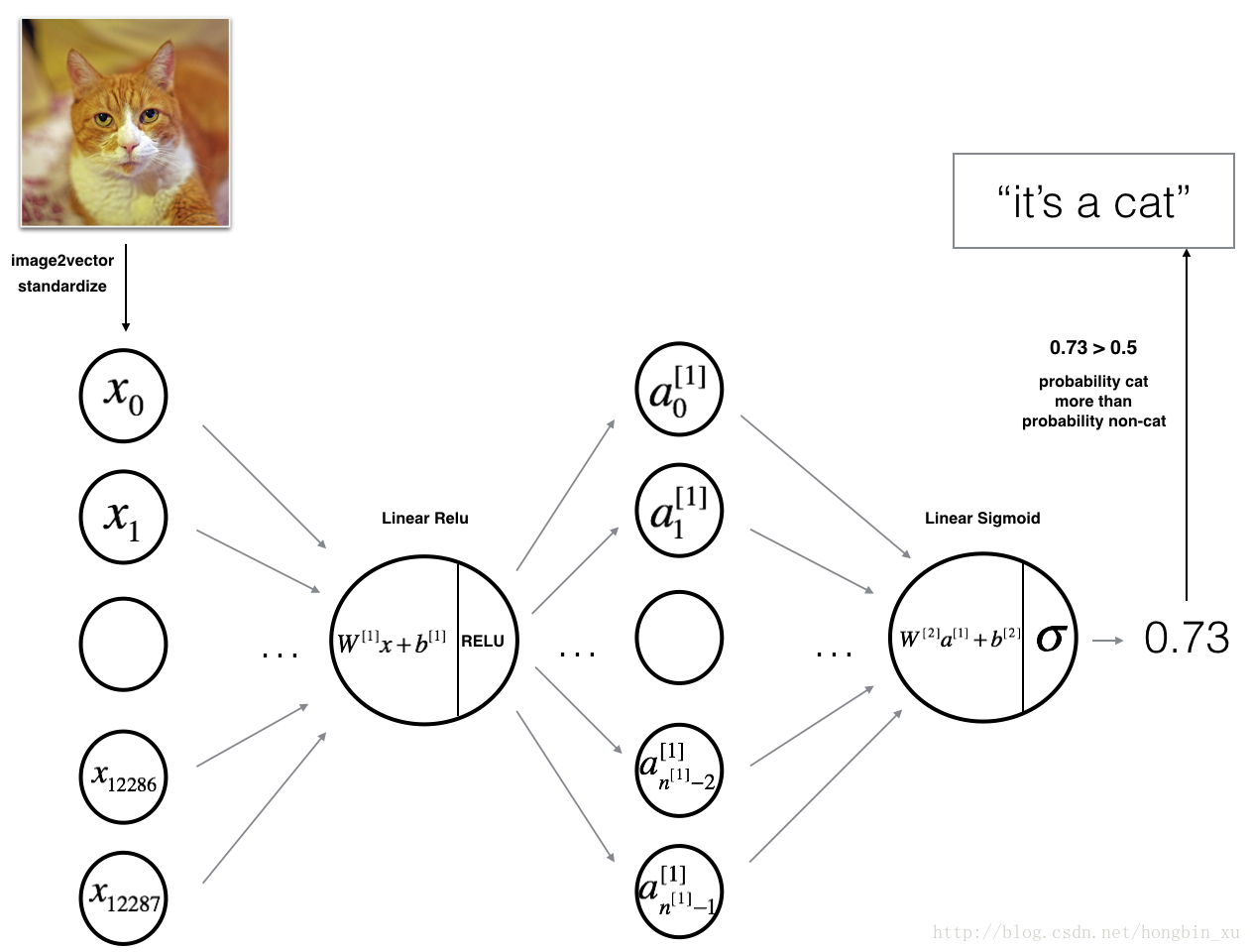
The model can be summarized as: INPUT -> LINEAR -> RELU -> LINEAR -> SIGMOID -> OUTPUT.

Detailed Architecture of figure 2:
- The input is a (64,64,3) image which is flattened to a vector of size (12288,1)$(12288,1)$.
- The corresponding vector: [x0,x1,...,x12287]T$[x_0,x_1,...,x_{12287}{]}^T$ is then multiplied by the weight matrix W[1]$W^{[1]}$ of size (n[1],12288)$(n^{[1]},12288)$.
- You then add a bias term and take its relu to get the following vector: [a[1]0,a[1]1,...,a[1]n[1]−1]T$[a_0^{[1]},a_1^{[1]},...,a_{n^{[1]}-1}^{[1]}{]}^T$.
- You then repeat the same process.
- You multiply the resulting vector by W[2]$W^{[2]}$ and add your intercept (bias).
- Finally, you take the sigmoid of the result. If it is greater than 0.5, you classify it to be a cat.

3.2 - L-layer deep neural network

It is hard to represent an L-layer deep neural network with the above representation. However, here is a simplified network representation:

Figure 3: L-layer neural network.
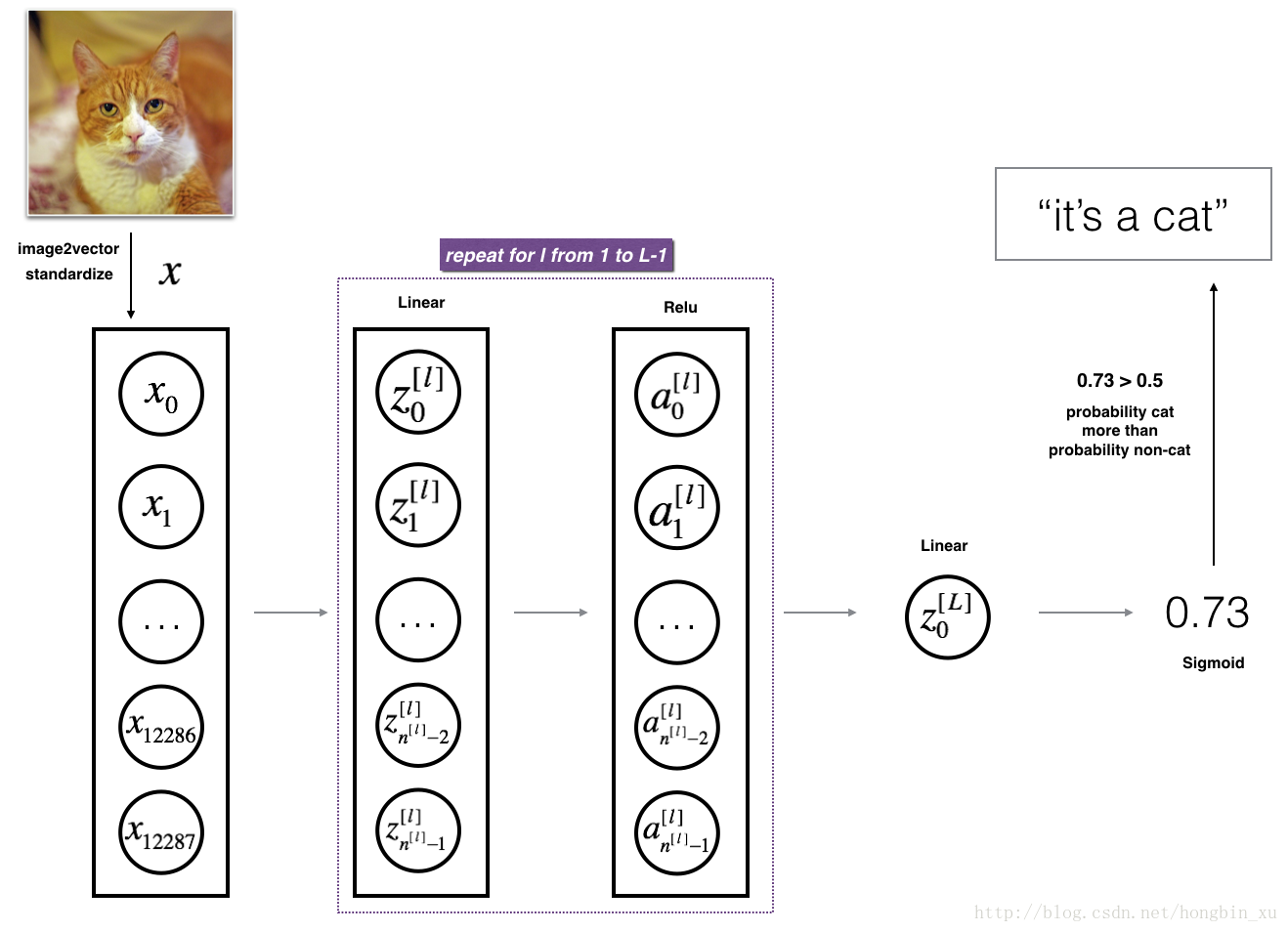
The model can be summarized as: [LINEAR -> RELU] ×$\times$ (L-1) -> LINEAR -> SIGMOID

Detailed Architecture of figure 3:
- The input is a (64,64,3) image which is flattened to a vector of size (12288,1).
- The corresponding vector: [x0,x1,...,x12287]T$[x_0,x_1,...,x_{12287}{]}^T$ is then multiplied by the weight matrix W[1]$W^{[1]}$ and then you add the intercept b[1]$b^{[1]}$. The result is called the linear unit.
- Next, you take the relu of the linear unit. This process could be repeated several times for each (W[l],b[l])$(W^{[l]},b^{[l]})$ depending on the model architecture.
- Finally, you take the sigmoid of the final linear unit. If it is greater than 0.5, you classify it to be a cat.

3.3 - General methodology

As usual you will follow the Deep Learning methodology to build the model:
1. Initialize parameters / Define hyperparameters
2. Loop for num_iterations:
a. Forward propagation
b. Compute cost function
c. Backward propagation
d. Update parameters (using parameters, and grads from backprop)
4. Use trained parameters to predict labels

Let’s now implement those two models!

4 - Two-layer neural network

Question: Use the helper functions you have implemented in the previous assignment to build a 2-layer neural network with the following structure: LINEAR -> RELU -> LINEAR -> SIGMOID. The functions you may need and their inputs are:

def initialize_parameters(n_x, n_h, n_y):
    ...
    return parameters 
def linear_activation_forward(A_prev, W, b, activation):
    ...
    return A, cache
def compute_cost(AL, Y):
    ...
    return cost
def linear_activation_backward(dA, cache, activation):
    ...
    return dA_prev, dW, db
def update_parameters(parameters, grads, learning_rate):
    ...
    return parameters

### CONSTANTS DEFINING THE MODEL ####
n_x = 12288     # num_px * num_px * 3
n_h = 7
n_y = 1
layers_dims = (n_x, n_h, n_y)

# GRADED FUNCTION: two_layer_model

def two_layer_model(X, Y, layers_dims, learning_rate = 0.0075, num_iterations = 3000, print_cost=False):
    """
    Implements a two-layer neural network: LINEAR->RELU->LINEAR->SIGMOID.

    Arguments:
    X -- input data, of shape (n_x, number of examples)
    Y -- true "label" vector (containing 0 if cat, 1 if non-cat), of shape (1, number of examples)
    layers_dims -- dimensions of the layers (n_x, n_h, n_y)
    num_iterations -- number of iterations of the optimization loop
    learning_rate -- learning rate of the gradient descent update rule
    print_cost -- If set to True, this will print the cost every 100 iterations 

    Returns:
    parameters -- a dictionary containing W1, W2, b1, and b2
    """

    np.random.seed(1)
    grads = {}
    costs = []                              # to keep track of the cost
    m = X.shape[1]                           # number of examples
    (n_x, n_h, n_y) = layers_dims

    # Initialize parameters dictionary, by calling one of the functions you'd previously implemented
    ### START CODE HERE ### (≈ 1 line of code)
    parameters = initialize_parameters(n_x, n_h, n_y)
    ### END CODE HERE ###

    # Get W1, b1, W2 and b2 from the dictionary parameters.
    W1 = parameters["W1"]
    b1 = parameters["b1"]
    W2 = parameters["W2"]
    b2 = parameters["b2"]

    # Loop (gradient descent)

    for i in range(0, num_iterations):

        # Forward propagation: LINEAR -> RELU -> LINEAR -> SIGMOID. Inputs: "X, W1, b1". Output: "A1, cache1, A2, cache2".
        ### START CODE HERE ### (≈ 2 lines of code)
        A1, cache1 = linear_activation_forward(X, W1, b1, "relu")
        A2, cache2 = linear_activation_forward(A1, W2, b2, "sigmoid")
        ### END CODE HERE ###

        # Compute cost
        ### START CODE HERE ### (≈ 1 line of code)
        cost = compute_cost(A2, Y)
        ### END CODE HERE ###

        # Initializing backward propagation
        dA2 = - (np.divide(Y, A2) - np.divide(1 - Y, 1 - A2))

        # Backward propagation. Inputs: "dA2, cache2, cache1". Outputs: "dA1, dW2, db2; also dA0 (not used), dW1, db1".
        ### START CODE HERE ### (≈ 2 lines of code)
        dA1, dW2, db2 = linear_activation_backward(dA2, cache2, "sigmoid")
        dA0, dW1, db1 = linear_activation_backward(dA1, cache1, "relu")
        ### END CODE HERE ###

        # Set grads['dWl'] to dW1, grads['db1'] to db1, grads['dW2'] to dW2, grads['db2'] to db2
        grads['dW1'] = dW1
        grads['db1'] = db1
        grads['dW2'] = dW2
        grads['db2'] = db2

        # Update parameters.
        ### START CODE HERE ### (approx. 1 line of code)
        parameters = update_parameters(parameters, grads, learning_rate)
        ### END CODE HERE ###

        # Retrieve W1, b1, W2, b2 from parameters
        W1 = parameters["W1"]
        b1 = parameters["b1"]
        W2 = parameters["W2"]
        b2 = parameters["b2"]

        # Print the cost every 100 training example
        if print_cost and i % 100 == 0:
            print("Cost after iteration {}: {}".format(i, np.squeeze(cost)))
        if print_cost and i % 100 == 0:
            costs.append(cost)

    # plot the cost

    plt.plot(np.squeeze(costs))
    plt.ylabel('cost')
    plt.xlabel('iterations (per tens)')
    plt.title("Learning rate =" + str(learning_rate))
    plt.show()

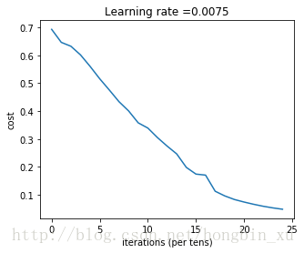
    return parameters

Run the cell below to train your parameters. See if your model runs. The cost should be decreasing. It may take up to 5 minutes to run 2500 iterations. Check if the “Cost after iteration 0” matches the expected output below, if not click on the square (⬛) on the upper bar of the notebook to stop the cell and try to find your error.

parameters = two_layer_model(train_x, train_y, layers_dims = (n_x, n_h, n_y), num_iterations = 2500, print_cost=True)

Cost after iteration 0: 0.693049735659989
Cost after iteration 100: 0.6464320953428849
Cost after iteration 200: 0.6325140647912678
Cost after iteration 300: 0.6015024920354665
Cost after iteration 400: 0.5601966311605748
Cost after iteration 500: 0.5158304772764731
Cost after iteration 600: 0.47549013139433255
Cost after iteration 700: 0.43391631512257495
Cost after iteration 800: 0.4007977536203886
Cost after iteration 900: 0.35807050113237976
Cost after iteration 1000: 0.3394281538366413
Cost after iteration 1100: 0.30527536361962654
Cost after iteration 1200: 0.2749137728213016
Cost after iteration 1300: 0.2468176821061484
Cost after iteration 1400: 0.19850735037466105
Cost after iteration 1500: 0.17448318112556638
Cost after iteration 1600: 0.17080762978096967
Cost after iteration 1700: 0.11306524562164705
Cost after iteration 1800: 0.09629426845937154
Cost after iteration 1900: 0.08342617959726867
Cost after iteration 2000: 0.07439078704319087
Cost after iteration 2100: 0.06630748132267934
Cost after iteration 2200: 0.05919329501038172
Cost after iteration 2300: 0.053361403485605606
Cost after iteration 2400: 0.04855478562877019

Expected Output:

**Cost after iteration 0**	0.6930497356599888
**Cost after iteration 100**	0.6464320953428849
**…**	…
**Cost after iteration 2400**	0.048554785628770206

Good thing you built a vectorized implementation! Otherwise it might have taken 10 times longer to train this.

Now, you can use the trained parameters to classify images from the dataset. To see your predictions on the training and test sets, run the cell below.

predictions_train = predict(train_x, train_y, parameters)

Accuracy: 1.0

Expected Output:

Accuracy

1.0

predictions_test = predict(test_x, test_y, parameters)

Accuracy: 0.72

Expected Output:

Accuracy

0.72

Note: You may notice that running the model on fewer iterations (say 1500) gives better accuracy on the test set. This is called “early stopping” and we will talk about it in the next course. Early stopping is a way to prevent overfitting.

Congratulations! It seems that your 2-layer neural network has better performance (72%) than the logistic regression implementation (70%, assignment week 2). Let’s see if you can do even better with an L$L$-layer model.

5 - L-layer Neural Network

Question: Use the helper functions you have implemented previously to build an L$L$-layer neural network with the following structure: [LINEAR -> RELU]×$\times$(L-1) -> LINEAR -> SIGMOID. The functions you may need and their inputs are:

def initialize_parameters_deep(layer_dims):
    ...
    return parameters 
def L_model_forward(X, parameters):
    ...
    return AL, caches
def compute_cost(AL, Y):
    ...
    return cost
def L_model_backward(AL, Y, caches):
    ...
    return grads
def update_parameters(parameters, grads, learning_rate):
    ...
    return parameters

### CONSTANTS ###
layers_dims = [12288, 20, 7, 5, 1] #  5-layer model

# GRADED FUNCTION: L_layer_model

def L_layer_model(X, Y, layers_dims, learning_rate = 0.0075, num_iterations = 3000, print_cost=False):#lr was 0.009
    """
    Implements a L-layer neural network: [LINEAR->RELU]*(L-1)->LINEAR->SIGMOID.

    Arguments:
    X -- data, numpy arr