Generative Adversarial Networks（生成對抗網路）

In 2014, Goodfellow et al. presented a method for training generative models called Generative Adversarial Networks (GANs for short). In a GAN, we build two different neural networks. Our first network is a traditional classification network, called the discriminator

. We will train the discriminator to take images, and classify them as being real (belonging to the training set) or fake (not present in the training set). Our other network, called the generator, will take random noise as input and transform it using a neural network to produce images. The goal of the generator is to fool the discriminator into thinking the images it produced are real.
在生成網路中，我們建立了兩個神經網路。第一個網路是典型的分類神經網路，稱為discriminator重點內容，我們訓練這個網路對影象進行識別，以區別真假的影象（真的圖片在訓練集當中，而假的則不在。另一個網路稱之為generator，它將隨機的噪聲作為輸入，將其轉化為使用神經網路訓練出來產生出來的影象，它的目的是混淆discriminator使其認為它生成的影象是真的。

We can think of this back and forth process of the generator (G$G$) trying to fool the discriminator (D$D$), and the discriminator trying to correctly classify real vs. fake as a minimax game:

minimizeGmaximizeDEx∼pdata[logD(x)]+Ez∼p(z)[log(1−D(G(z)))]$$\underset{G}{\text{minimize}}\underset{D}{\text{maximize}}{\mathbb{E}}_{x\sim p_{\text{data}}}\left[\log D(x)\right]+{\mathbb{E}}_{z\sim p(z)}\left[\log \left(1-D(G(z))\right)\right]$$

where z∼p(z)$z\sim p(z)$ are the random noise samples, G(z)$G(z)$ are the generated images using the neural network generator G$G$, and D$D$ is the output of the discriminator, specifying the probability of an input being real. In Goodfellow et al., they analyze this minimax game and show how it relates to minimizing the Jensen-Shannon divergence between the training data distribution and the generated samples from G$G$.

To optimize this minimax game, we will alternate between taking gradient descent steps on the objective for G$G$, and gradient ascent steps on the objective for D$D$:
1. update the generator (G$G$) to minimize the probability of the discriminator making the correct choice.
2. update the discriminator (D$D$) to maximize the probability of the discriminator making the correct choice.

While these updates are useful for analysis, they do not perform well in practice. Instead, we will use a different objective when we update the generator: maximize the probability of the discriminator making the incorrect choice. This small change helps to allevaiate problems with the generator gradient vanishing when the discriminator is confident. This is the standard update used in most GAN papers, and was used in the original paper from Goodfellow et al..

In this assignment, we will alternate the following updates:
在這項任務中，我們將輪換執行以下的更新：
1. Update the generator (G$G$) to maximize the probability of the discriminator making the incorrect choice on generated data:
更新generator (G$G$)以最大化discriminator做出錯誤分類的概率。

maximizeGEz∼p(z)[logD(G(z))]$$\underset{G}{\text{maximize}}{\mathbb{E}}_{z\sim p(z)}\left[\log D(G(z))\right]$$
2. Update the discriminator (D$D$), to maximize the probability of the discriminator making the correct choice on real and generated data:
更新discriminator (D$D$)以最大化discriminator做出正確分類的概率。
maximizeDEx∼pdata[logD(x)]+Ez∼p(z)[log(1−D(G(z)))]$$\underset{D}{\text{maximize}}{\mathbb{E}}_{x\sim p_{\text{data}}}\left[\log D(x)\right]+{\mathbb{E}}_{z\sim p(z)}\left[\log \left(1-D(G(z))\right)\right]$$

What else is there?

Since 2014, GANs have exploded into a huge research area, with massive workshops, and hundreds of new papers. Compared to other approaches for generative models, they often produce the highest quality samples but are some of the most difficult and finicky models to train (see this github repo that contains a set of 17 hacks that are useful for getting models working). Improving the stabiilty and robustness of GAN training is an open research question, with new papers coming out every day! For a more recent tutorial on GANs, see here. There is also some even more recent exciting work that changes the objective function to Wasserstein distance and yields much more stable results across model architectures: WGAN, WGAN-GP.

GANs are not the only way to train a generative model! For other approaches to generative modeling check out the deep generative model chapter of the Deep Learning book. Another popular way of training neural networks as generative models is Variational Autoencoders (co-discovered here and here). Variatonal autoencoders combine neural networks with variationl inference to train deep generative models. These models tend to be far more stable and easier to train but currently don’t produce samples that are as pretty as GANs.

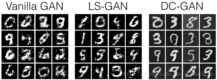
Here’s an example of what your outputs from the 3 different models you’re going to train should look like… note that GANs are sometimes finicky, so your outputs might not look exactly like this… this is just meant to be a rough guideline of the kind of quality you can expect:

程式講解：

1、載入所需要的模組和庫，設定展示圖片函式以及其他對影象預處理函式

import torch
import torch.nn as nn
from torch.nn import init
from torch.autograd import Variable
import torchvision
import torchvision.transforms as T
import torch.optim as optim
from torch.utils.data import DataLoader
from torch.utils.data import sampler
import torchvision.datasets as dset

import numpy as np

import matplotlib.pyplot as plt
import matplotlib.gridspec as gridspec

%matplotlib inline
plt.rcParams['figure.figsize'] = (10.0, 8.0) # set default size of plots
plt.rcParams['image.interpolation'] = 'nearest'
plt.rcParams['image.cmap'] = 'gray'

def show_images(images):
    images = np.reshape(images, [images.shape[0], -1])  # images reshape to (batch_size, D)
    sqrtn = int(np.ceil(np.sqrt(images.shape[0])))
    sqrtimg = int(np.ceil(np.sqrt(images.shape[1])))

    fig = plt.figure(figsize=(sqrtn, sqrtn))
    gs = gridspec.GridSpec(sqrtn, sqrtn)
    gs.update(wspace=0.05, hspace=0.05)

    for i, img in enumerate(images):
        ax = plt.subplot(gs[i])
        plt.axis('off')
        ax.set_xticklabels([])
        ax.set_yticklabels([])
        ax.set_aspect('equal')
        plt.imshow(img.reshape([sqrtimg,sqrtimg]))
    return 

def preprocess_img(x):
    return 2 * x - 1.0

def deprocess_img(x):
    return (x + 1.0) / 2.0

def rel_error(x,y):
    return np.max(np.abs(x - y) / (np.maximum(1e-8, np.abs(x) + np.abs(y))))

def count_params(model):
    """Count the number of parameters in the current TensorFlow graph """
    param_count = np.sum([np.prod(p.size()) for p in model.parameters()])
    return param_count

answers = np.load('gan-checks-tf.npz')

採用的資料集

因為GANS中超引數的設定非常非常麻煩，同樣也需要很多的訓練epoch。為了加快訓練速度，這裡使用MNIST資料集，擁有60，000個訓練集和10，000測試集。每個圖片中包含一個數字（0-9，背景為黑色，數字為白色）。這個資料集通過標準神經網路的訓練已經可以達到超過99%的準確率。

這裡使用pytorch中自帶的資料集工具進行對資料的提取：

# 取樣函式為自己定義的序列取樣（即按順序取樣）
class ChunkSampler(sampler.Sampler): 
    """Samples elements sequentially from some offset. 
    Arguments:
        num_samples: # of desired datapoints
        start: offset where we should start selecting from
    """
    def __init__(self, num_samples, start=0):
        self.num_samples = num_samples
        self.start = start

    def __iter__(self):
        return iter(range(self.start, self.start + self.num_samples))

    def __len__(self):
        return self.num_samples

NUM_TRAIN = 50000   # 訓練集數量
NUM_VAL = 5000      # 測試集數量

NOISE_DIM = 96      
batch_size = 128

mnist_train = dset.MNIST('./cs231n/datasets/MNIST_data', train=True, download=True,
                           transform=T.ToTensor())
loader_train = DataLoader(mnist_train, batch_size=batch_size,
                          sampler=ChunkSampler(NUM_TRAIN, 0)) # 從0位置開始取樣NUM_TRAIN個數

mnist_val = dset.MNIST('./cs231n/datasets/MNIST_data', train=True, download=True,
                           transform=T.ToTensor())
loader_val = DataLoader(mnist_val, batch_size=batch_size,
                        sampler=ChunkSampler(NUM_VAL, NUM_TRAIN)) # 從NUM_TRAIN位置開始取樣NUM_VAL個數


imgs = loader_train.__iter__().next()[0].view(batch_size, 784).numpy().squeeze()
show_images(imgs)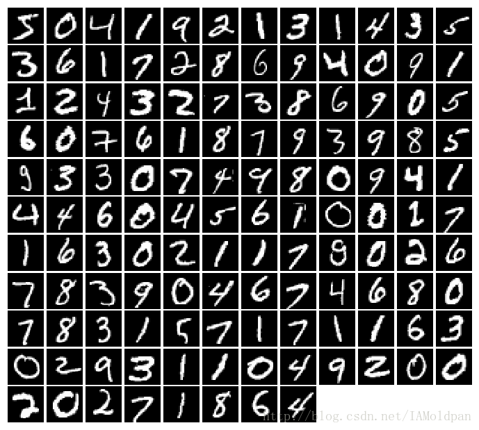

Random Noise

Generate uniform noise from -1 to 1 with shape [batch_size, dim].
這裡產生一個從-1 - 1的均勻噪聲函式，形狀為 [batch_size, dim].

def sample_noise(batch_size, dim):
    """
    Generate a PyTorch Tensor of uniform random noise.

    Input:
    - batch_size: Integer giving the batch size of noise to generate.
    - dim: Integer giving the dimension of noise to generate.

    Output:
    - A PyTorch Tensor of shape (batch_size, dim) containing uniform
      random noise in the range (-1, 1).
    """
    temp = torch.rand(batch_size, dim) + torch.rand(batch_size, dim)*(-1)

    return temp

接下來定義平鋪函式和反平鋪函式，用於對影象中資料的處理

class Flatten(nn.Module):
    def forward(self, x):
        N, C, H, W = x.size() # read in N, C, H, W
        return x.view(N, -1)  # "flatten" the C * H * W values into a single vector per image

class Unflatten(nn.Module):
    """
    An Unflatten module receives an input of shape (N, C*H*W) and reshapes it
    to produce an output of shape (N, C, H, W).
    """
    def __init__(self, N=-1, C=128, H=7, W=7):
        super(Unflatten, self).__init__()
        self.N = N
        self.C = C
        self.H = H
        self.W = W
    def forward(self, x):
        return x.view(self.N, self.C, self.H, self.W)

def initialize_weights(m):
    if isinstance(m, nn.Linear) or isinstance(m, nn.ConvTranspose2d):
        init.xavier_uniform(m.weight.data)

前期工作準備好了，開始寫discriminator函式：

discriminator神經網路即去判斷generator產生的影象是否為假，同時判斷正確的影象是否為真，包含的網路層為：

Fully connected layer from size 784 to 256
LeakyReLU with alpha 0.01
Fully connected layer from 256 to 256
LeakyReLU with alpha 0.01
Fully connected layer from 256 to 1

我們使用LeakyRelu，設定其alpha引數為0.01
該判別器的輸出應該為[batch_size, 1], 每個batch中包含正確分類.

def discriminator():
    """
    Build and return a PyTorch model implementing the architecture above.
    """
    model = nn.Sequential(
        Flatten(),
        nn.Linear(784,256),
        nn.LeakyReLU(0.01, inplace=True),
        nn.Linear(256,256),
        nn.LeakyReLU(0.01, inplace=True),
        nn.Linear(256,1)
    )
    return model

Generator

寫生成網路:
Fully connected layer from noise_dim to 1024
ReLU
Fully connected layer with size 1024
ReLU
Fully connected layer with size 784
TanH（To clip the image to be [-1,1]）

def generator(noise_dim=NOISE_DIM):
    """
    Build and return a PyTorch model implementing the architecture above.
    """
    model = nn.Sequential(
        nn.Linear(noise_dim, 1024),
        nn.ReLU(inplace=True),
        nn.Linear(1024, 1024),
        nn.ReLU(inplace=True),
        nn.Linear(1024, 784),
        nn.Tanh(),
    )
    return model

GAN Loss

Compute the generator and discriminator loss. The generator loss is:

ℓG=−Ez∼p(z)[logD(G(z))]$${\ell }_G=-{\mathbb{E}}_{z\sim p(z)}\left[\log D(G(z))\right]$$
and the discriminator loss is:

相關推薦

利用pytorch實現GAN(生成對抗網路)-MNIST影象-cs231n-assignment3

Generative Adversarial Networks（生成對抗網路） In 2014, Goodfellow et al. presented a method for training generative models called Ge

【深度學習】GAN生成對抗網路原理詳解（1）

一個 GAN 框架，最少（但不限於）擁有兩個組成部分，一個是生成模型 G，一個是判別模型 D。在訓練過程中，會把生成模型生成的樣本和真實樣本隨機地傳送一張（或者一個 batch）給判別模型 D。判別模型 D 的目標是儘可能正確地識別出真實樣本（輸出為“真”，或者1），和儘可能

Generative Adversarial Network (GAN) 生成對抗網路

Part One. Introduction of GAN The Structure of GAN 其中可以看到GAN中有兩個最關鍵的結構就是generator（生成器）和discriminator（判別器）。生成器是為了生成接近真實資料分佈的虛假樣本，判別器是為了

GAN-生成對抗網路原理

最近一直在看GAN，我一直認為只有把部落格看了一遍，然後再敲一遍。這樣才會有深刻的感悟。   GAN（生成式對抗網路）（GAN, Generative Adversarial Networks ）是一種深度學習模型，分佈在無監督學習上。 分成兩個模組：生成模型（Generative

tensorflow 1.01中GAN(生成對抗網路)手寫字型生成例子(MINST)的測試

為了更好地掌握GAN的例子，從網上找了段程式碼進行跑了下，測試了效果。具體過程如下： 程式碼檔案如下： import tensorflow as tf from tensorflow.examples.tutorials.mnist import input_data i

GAN|生成對抗網路的前沿進展（論文、框架&資源）全面總結

成模型（GenerativeModel）是一種可以通過學習訓練樣本來產生更多類似樣本的模型。在所有生成模型當中，最具潛力的是生成對抗網路（Generative Adversarial Networks, GANs）。GANs 是非監督機器學習的一種，它的運作方式可被看做

GAN—生成對抗網路

原理： 假設我們有兩個網路：一個生G（Generator），一個判別D（Discriminator）。 G是一個生成圖片的的網路，它接受一個隨機的噪聲z，通過這個噪聲生成圖片，記做G（z）。 D是一個判別網路，判斷一張圖片是不是“真實的”。它的輸入引數是x

生成對抗網路消除影象模糊（Keras）

2017年，烏克蘭天主教大學、布拉格捷克理工大學和解決方案提供商Eleks聯手公佈了一篇論文，文章標題為《DeblurGAN: Blind Motion Deblurring Using Conditi

keras 實現GAN（生成對抗網路）

本文將介紹如何在Keras中以最小的形式實現GAN。具體實現是一個深度卷積GAN，或DCGAN：一個GAN，其中generator和discriminator是深度卷積網路，它利用`Conv2DTranspose`層對generator中的影象上取樣。 然後將在CIFAR10的影象上訓練GAN，CI

用pytorch實現GAN——mnist（含有全部註釋和網路思想）

#coding=utf-8 import torch.autograd import torch.nn as nn from torch.autograd import Variable from torchvision import transforms from torchvision impo

一篇讀懂生成對抗網路（GAN）原理+tensorflow程式碼實現

作者：JASON 2017.10.15   生成對抗網路GAN（Generative adversarial networks）是最近很火的深度學習方法，要理解它可以把它分成生成模型和判別模型兩個部分，簡單來說就是：兩個人比賽，看是 A 的矛厲害，還是 B

生成對抗網路GAN---生成mnist手寫數字影象示例（附程式碼）

Ian J. Goodfellow等人於2014年在論文Generative Adversarial Nets中提出了一個通過對抗過程估計生成模型的新框架。框架中同時訓練兩個模型：一個生成模型（generative model）G，用來捕獲資料分佈；一個判別模型(discri

七個不容易被發現的生成對抗網路（GAN）用例

像許多追隨AI發展的人一樣，我無法忽略生成建模的最新進展，尤其是影象生成中生成對抗網路（GAN）的巨大成功。看看下面這些樣本：它們與真實照片幾乎沒有區別！   從2014年到2018年，面部生成的進展也非常顯著。 這些結果讓我感到興奮，但我內心總是懷疑它們是否真

生成對抗網路（GAN）應用於影象分類

　　近年來，深度學習技術被廣泛應用於各類資料處理任務中，比如影象、語音和文字。而生成對抗網路（GAN）和強化學習（RL）已經成為了深度學習框架中的兩顆“明珠”。強化學習主要用於決策問題，主要的應用就是遊戲，比如deepmind團隊的AlphaGo。因為我的研究方向是影象的有監督分類問題，

洞見 | 生成對抗網路GAN最近在NLP領域有哪些應用

分享一下我老師大神的人工智慧教程！零基礎，通俗易懂！http://blog.csdn.net/jiangjunshow 也歡迎大家轉載本篇文章。分享知識，造福人民，實現我們中華民族偉大復興！        

初步認識GAN（生成對抗網路）

初步認識GAN（生成對抗網路） 1.GAN的發明 生成模型的基本思想是輸入一個訓練樣本集合，形成樣本概率分佈的表徵。 常用的生成模型是直接推斷他的密度概率函式。 好的生成模型有以下幾方面的實際應用; 1. 提升圖片的質量（高解析度） 2. 預測未來狀態的規劃 3.生成缺失資料和標

生成對抗網路GAN資料打包分享

  全文摘要 生成式對抗網路，即所謂的GAN是近些年來最火的無監督學習方法之一，模型由Goodfellow等人在2014年首次提出，將博弈論中非零和博弈思想與生成模型結合在一起，巧妙避開了傳統生成模型中概率密度估計困難等問題，是生成模型達到良好的效果。本文總結收集了

生成對抗網路學習（GAN）學習筆記

文章目錄 2018-11-16 GAN的原理 2018-11-15 Multimodal Unsupervised Image-to-Image Translation 2018-11-13 Image-to-

在瀏覽器中進行深度學習：TensorFlow.js (八）生成對抗網路 （GAN

Generative Adversarial Network 是深度學習中非常有趣的一種方法。GAN最早源自Ian Goodfellow的這篇論文。LeCun對GAN給出了極高的評價： “There are many interesting recent development in deep learni

生成對抗網路GAN系列（六）--- CycleGAN---文末附程式碼

Unpaired Image-to-Image Translation using Cycle-Consistent Adversarial Networks Jun-Yan Zhu      Taesung Park          Phillip Isola