
logistic迴歸報錯問題:Warning messages: 1: glm.fit:演算法沒有聚合 2: glm.fit:擬合機率算出來是數值零或一
logistic迴歸的時候報錯問題包括下面兩種
Warning: glm.fit: algorithm did not converge
Warning: glm.fit: fitted probabilities numerically 0 or 1 occurred
Warning messages:
1: glm.fit:演算法沒有聚合
2: glm.fit:擬合機率算出來是數值零或一
做logistic迴歸的時候這個問題比較常見,下面來舉例,為什麼會出現這些問題。
首先是glm函式介紹:
glm(formula, family=family.generator, data,control = list(...))
family:每一種響應分佈(指數分佈族)允許各種關聯函式將均值和線性預測器關聯起來。
常用的family:
binomal(link='logit') ----響應變數服從二項分佈,連線函式為logit,即logistic迴歸
binomal(link='probit') ----響應變數服從二項分佈,連線函式為probit
poisson(link='identity') ----響應變數服從泊松分佈,即泊松迴歸
control:控制演算法誤差和最大迭代次數
glm.control(epsilon = 1e-8, maxit = 25, trace = FALSE)
-----maxit:演算法最大迭代次數,改變最大迭代次數:control=list(maxit=100)
glm函式使用:
library("ggplot2")
data<-iris[1:100,]
samp<-sample(100,80)
names(data)<-c('sl','sw','pl','pw','species')
testdata<-data[samp,]
traindata<-data[-samp,]
lgst<-glm(testdata$species~pl,binomial(link='logit'),data=testdata)
## Warning: glm.fit: algorithm did not converge## Warning: glm.fit: fitted probabilities numerically 0 or 1 occurredsummary(lgst)##
## Call:
## glm(formula = testdata$species ~ pl, family = binomial(link = "logit"),
## data = testdata)
##
## Deviance Residuals:
## Min 1Q Median 3Q Max
## -2.202e-05 -2.100e-08 -2.100e-08 2.100e-08 3.233e-05
##
## Coefficients:
## Estimate Std. Error z value Pr(>|z|)
## (Intercept) -97.30 87955.20 -0.001 0.999
## pl 39.56 34756.04 0.001 0.999
##
## (Dispersion parameter for binomial family taken to be 1)
##
## Null deviance: 1.1045e+02 on 79 degrees of freedom
## Residual deviance: 2.0152e-09 on 78 degrees of freedom
## AIC: 4
##
## Number of Fisher Scoring iterations: 25注意在使用glm函式就行logistic迴歸時,出現警告:
Warning messages:
1: glm.fit:演算法沒有聚合
2: glm.fit:擬合機率算出來是數值零或一
同時也可以發現兩個係數的P值都為0.999,說明迴歸係數不顯著。
第一個警告:演算法不收斂。
由於在進行logistic迴歸時,依照極大似然估計原則進行迭代求解迴歸係數,glm函式預設的最大迭代次數 maxit=25,當資料不太好時,經過25次迭代可能演算法 還不收斂,所以可以通過增大迭代次數嘗試解決演算法不收斂的問題。但是當增大迭代次數後演算法仍然不收斂,此時資料就是真的不好了,需要對資料進行奇異值檢驗等進一步的處理。
lgst<-glm(testdata$species~pl,binomial(link='logit'),data=testdata,control=list(maxit=100))## Warning: glm.fit: fitted probabilities numerically 0 or 1 occurredsummary(lgst)##
## Call:
## glm(formula = testdata$species ~ pl, family = binomial(link = "logit"),
## data = testdata, control = list(maxit = 100))
##
## Deviance Residuals:
## Min 1Q Median 3Q Max
## -8.134e-06 -2.110e-08 -2.110e-08 2.110e-08 1.204e-05
##
## Coefficients:
## Estimate Std. Error z value Pr(>|z|)
## (Intercept) -106.14 237658.98 0 1
## pl 43.16 93735.01 0 1
##
## (Dispersion parameter for binomial family taken to be 1)
##
## Null deviance: 1.1070e+02 on 79 degrees of freedom
## Residual deviance: 2.7741e-10 on 78 degrees of freedom
## AIC: 4
##
## Number of Fisher Scoring iterations: 27如上,通過增加迭代次數,解決了第一個警告,此時演算法收斂。
但是第二個警告仍然存在,且迴歸係數P=1,仍然不顯著。
第二個警告:擬合概率算出來的概率為0或1
首先,這個警告是什麼意思?
我們先來看看訓練樣本的logist迴歸結果,擬合出的每個樣本屬於'setosa'類的概率為多少?
lgst<-glm(testdata$species~pl,binomial(link='logit'),data=testdata,control=list(maxit=100))## Warning: glm.fit: fitted probabilities numerically 0 or 1 occurredp<-predict(lgst,type='response')
qplot(seq(-2,2,length=80),sort(p),col='predict')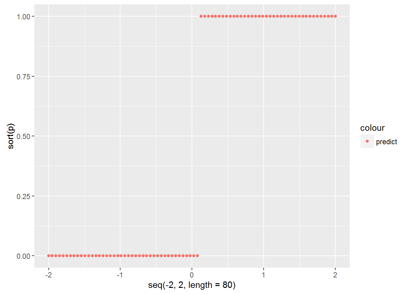
可以看出訓練樣本為'setosa'類的概率不是幾乎為0,就是幾乎為1,並不是我們預想中的logistic模型的S型曲線,這就是第二個警告的意思。
那麼問題來了,為什麼會出現這種情況?
(以下內容只是本人蔘考一些解釋的個人理解)
這種情況的出現可以理解為一種過擬合,由於資料的原因,在迴歸係數的優化搜尋過程中,使得分類的種類屬於某一種類(y=1)的線性擬合值趨於大,分類種類為另一 類(y=0)的線性擬合值趨於小。
由於在求解迴歸係數時,使用的是極大似然估計的原理,即迴歸係數在搜尋過程中使得似然函式極大化:

所以在搜尋過程中偏向於使得y=1的h(x)趨向於大,而使得y=0的h(x)趨向於小。

即係數Θ使得 Y=1類的 -ΘTX 趨向於大,使得Y=0類的 -ΘTX 趨向於小。而這樣的結果就會導致P(y=1|x;Θ)-->1 ; P(y=0|x;Θ)-->0 .
那麼問題又來了,什麼樣的資料會導致這樣的過擬合產生呢?
先來看看上述logistic迴歸中種類為setosa和versicolor的樣本pl值的情況。(橫軸代表pl值,為了避免樣本pl資料點疊加在一起,增加了一個無關的y值使樣本點展開)
testdata$y <- c(1:80)
qplot(pl,y,data =testdata,colour =factor(species))
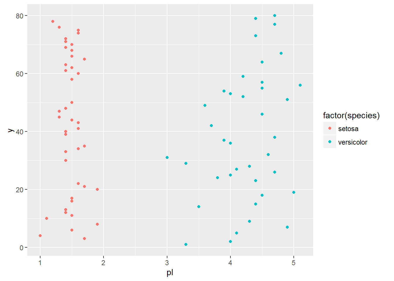
可以看出兩類資料明顯的完全線性可分。
故在迴歸係數搜尋過程中只要使得一元線性函式h(x)的斜率的絕對值偏大,就可以實現y=1類的h(x)趨向大,y=0類的h(x)趨向小。
所以當樣本資料完全可分時,logistic迴歸往往會導致過擬合的問題,即出現第二個警告:擬合概率算出來的概率為0或1。
出現了第二個警告後的logistic模型進行預測時往往是不適用的,對於這種線性可分的樣本資料,其實直接使用規則判斷的方法則簡單且適用(如當pl<2.5時則直接判斷為setosa類,pl>2.5時判斷為versicolor類)。
以下,對於不完全可分的二維訓練資料展示logistic迴歸過程。
data<-iris[51:150,]
samp<-sample(100,80)
names(data)<-c('sl','sw','pl','pw','species')
testdata<-data[samp,]
traindata<-data[-samp,]
lgst<-glm(testdata$species~sw+pw,binomial(link='logit'),data=testdata)
summary(lgst)
##
## Call:
## glm(formula = testdata$species ~ sw + pw, family = binomial(link = "logit"),
## data = testdata)
##
## Deviance Residuals:
## Min 1Q Median 3Q Max
## -1.68123 -0.12839 -0.01807 0.07783 2.24191
##
## Coefficients:
## Estimate Std. Error z value Pr(>|z|)
## (Intercept) -12.792 5.828 -2.195 0.028168 *
## sw -4.214 1.970 -2.139 0.032432 *
## pw 15.229 3.984 3.823 0.000132 ***
## ---
## Signif. codes: 0 '***' 0.001 '**' 0.01 '*' 0.05 '.' 0.1 ' ' 1
##
## (Dispersion parameter for binomial family taken to be 1)
##
## Null deviance: 110.854 on 79 degrees of freedom
## Residual deviance: 21.382 on 77 degrees of freedom
## AIC: 27.382
##
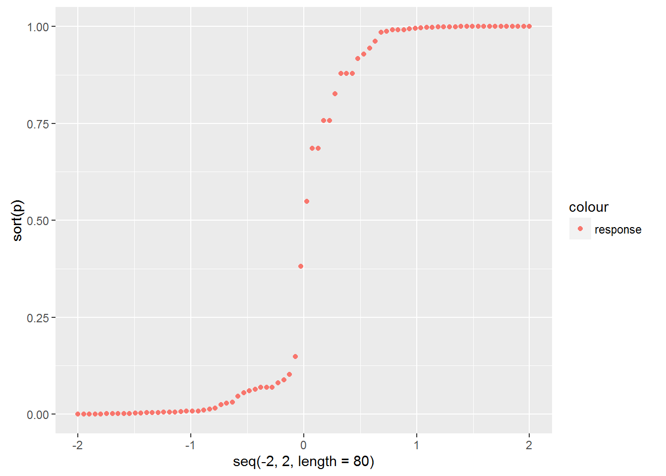
## Number of Fisher Scoring iterations: 7擬合概率曲線圖:(基本上符合logistic模型的S型曲線)
p<-predict(lgst,type='response')
qplot(seq(-2,2,length=80),sort(p),col="response")
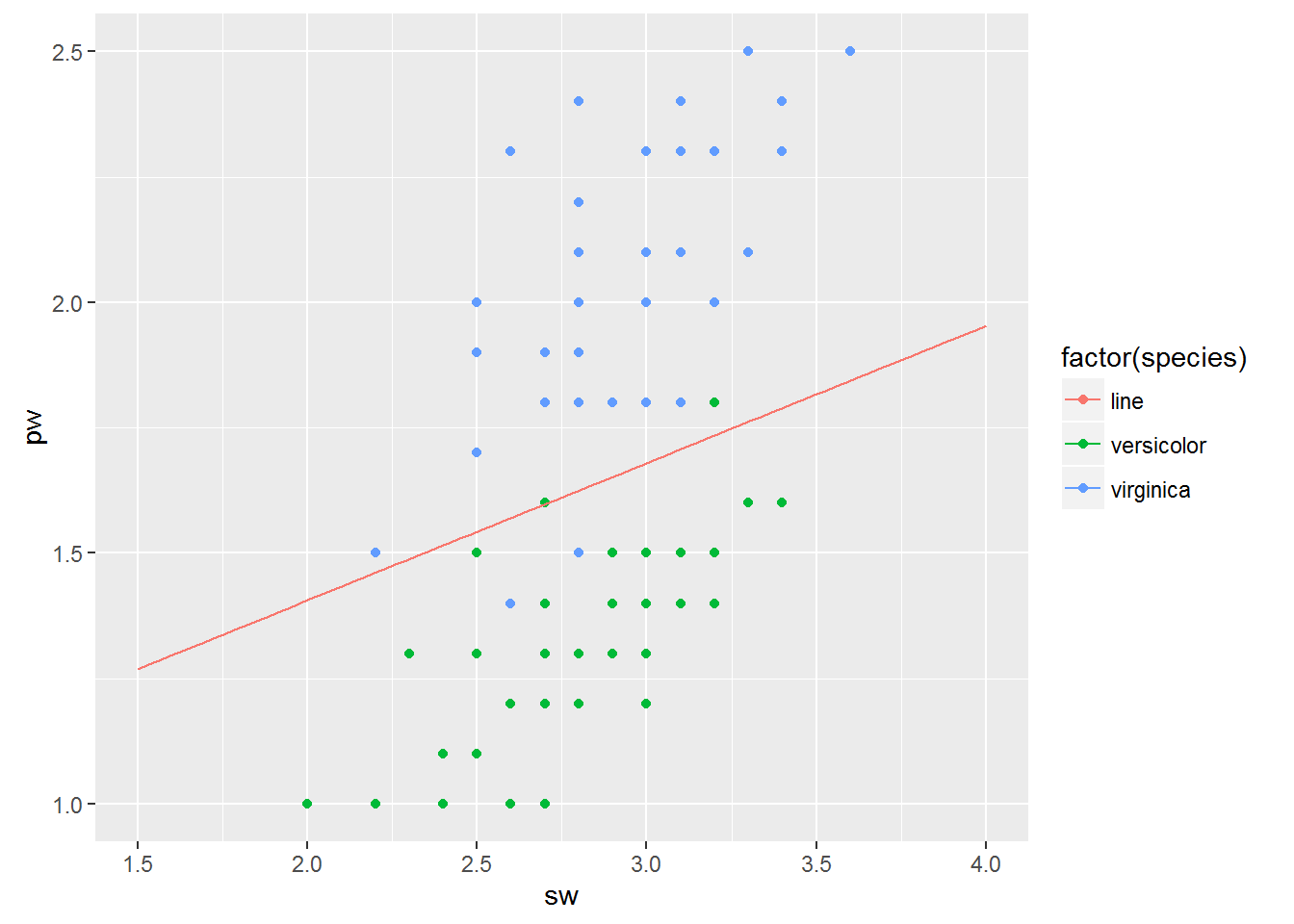
訓練樣本散點圖及分類邊界:
(畫logistic迴歸的分類邊界即畫曲線h(x)=0.5)
x3<-seq(1.5,4,length=80)
y3<-(4.284/15.656)*x3+13.447/15.656
aaa<-data.frame(x3,y3)

p <- ggplot()
p+geom_point(data = testdata,aes(x=sw,y=pw,colour=factor(species)))+
geom_line(data = aaa,aes(x = x3,y = y3,colour="line"))
內容參考於原博主,為加深印象,我自己做了一遍,圖換成了ggplot2,原文參考如下連線: