Ian Meyers is a Solutions Architecture Senior Manager with AWS
Zach Christopherson, an Amazon Redshift Database Engineer, contributed to this post

Amazon Redshift is a fully managed, petabyte scale, massively parallel data warehouse that offers simple operations and high performance. Customers use Amazon Redshift for everything from accelerating existing database environments that are struggling to scale, to ingestion of web logs for big data analytics use cases. Amazon Redshift provides an industry standard JDBC/ODBC driver interface, which allows customers to connect their existing business intelligence tools and re-use existing analytics queries.

Amazon Redshift can run any type of data model, from a production transaction system third-normal-form model, to star and snowflake schemas, or simple flat tables. As customers adopt Amazon Redshift, they must consider its architecture in order to ensure that their data model is correctly deployed and maintained by the database. This post takes you through the most common issues that customers find as they adopt Amazon Redshift, and gives you concrete guidance on how to address each. If you address each of these items, you should be able to achieve optimal performance of queries and so scale effectively to meet customer demand.

Issue #1: Incorrect column encoding

Amazon Redshift is a column-oriented database, which means that rather than organising data on disk by rows, data is stored by column, and rows are extracted from column storage at runtime. This architecture is particularly well suited to analytics queries on tables with a large number of columns, where most queries only access a subset of all possible dimensions and measures. Amazon Redshift is able to only access those blocks on disk that are for columns included in the SELECT or WHERE clause, and doesn’t have to read all table data to evaluate a query. Data stored by column should also be encoded (see

Running an Amazon Redshift cluster without column encoding is not considered a best practice, and customers find large performance gains when they ensure that column encoding is optimally applied. To determine if you are deviating from this best practice, you can use the v_extended_table_info view from the Amazon Redshift Utils GitHub repository. Create the view, and then run the following query to determine if any tables have columns with no encoding applied:

SELECT database, tablename, columns 
FROM admin.v_extended_table_info 
ORDER BY database;

Afterward, review the tables and columns which aren’t encoded by running the following query:

SELECT trim(n.nspname || '.' || c.relname) AS "table",
  trim(a.attname) AS "column",
  format_type(a.atttypid, a.atttypmod) AS "type", 
  format_encoding(a.attencodingtype::integer) AS "encoding", 
  a.attsortkeyord AS "sortkey"
FROM pg_namespace n, pg_class c, pg_attribute a 
WHERE n.oid = c.relnamespace 
AND c.oid = a.attrelid 
AND a.attnum > 0 
AND NOT a.attisdropped and n.nspname NOT IN ('information_schema','pg_catalog','pg_toast') 
AND format_encoding(a.attencodingtype::integer) = 'none' 
AND c.relkind='r' 
AND a.attsortkeyord != 1 
ORDER BY n.nspname, c.relname, a.attnum;

If you find that you have tables without optimal column encoding, then use the Amazon Redshift Column Encoding Utility from the Utils repository to apply encoding. This command line utility uses the ANALYZE COMPRESSION command on each table. If encoding is required, it generates a SQL script which creates a new table with the correct encoding, copies all the data into the new table, and then transactionally renames the new table to the old name while retaining the original data. (Please note that the first column in a compound sort key should not be encoded, and is not encoded by this utility.)

Issue #2 – Skewed table data

Amazon Redshift is a distributed, shared nothing database architecture where each node in the cluster stores a subset of the data. Each node is further subdivided into slices, with each slice having one or more dedicated cores. The number of slices per node depends on the node type of the cluster. For example, each DS2.XL compute node has two slices, and each DS2.8XL compute node has 16 slices. When a table is created, you decide whether to spread the data evenly among slices (default), or assign data to specific slices on the basis of one of the columns. By choosing columns for distribution that are commonly joined together, you can minimize the amount of data transferred over the network during the join. This can significantly increase performance on these types of queries.

The selection of a good distribution key is the topic of many AWS articles, including Choose the Best Distribution Style; see a definitive guide to distribution and sorting of star schemas in the Optimizing for Star Schemas and Interleaved Sorting on Amazon Redshift blog post. In general, a good distribution key should exhibit the following properties:

• High cardinality – There should be a large number of unique data values in the column relative to the number of slices in the cluster.
• Uniform distribution/low skew – Ideally, each unique value in the distribution key column should occur in the table about the same number of times. This allows Amazon Redshift to put the same number of records on each slice in the cluster.
• Commonly joined – The column in a distribution key should be one that you usually join to other tables. If you have many possible columns that fit this criterion, then you may choose the column that joins the largest number of rows at runtime (this is usually, but not always, the column that joins to the largest table).

A skewed distribution key results in slices not working equally hard as each other during query execution, requiring unbalanced CPU or memory, and ultimately only running as fast as the slowest slice:

If skew is a problem, you typically see that node performance is uneven on the cluster. Use one of the admin scripts in the Amazon Redshift Utils GitHub repository, such as table_inspector.sql, to see how data blocks in a distribution key map to the slices and nodes in the cluster.

If you find that you have tables with skewed distribution keys, then consider changing the distribution key to a column that exhibits high cardinality and uniform distribution. Evaluate a candidate column as a distribution key by creating a new table using CTAS:

CREATE TABLE my_test_table DISTKEY (<column name>) AS SELECT <column name> FROM <table name>;

Run the table_inspector.sql script against the table again to analyze data skew.

If there is no good distribution key in any of your records, you may find that moving to EVEN distribution works better. For small tables (for example, dimension tables with a couple of million rows), you can also use DISTSTYLE ALL to place table data onto the first slice of every node in the cluster.

Issue #3 – Queries not benefiting from sort keys

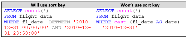
Amazon Redshift tables can have a sort key column identified, which acts like an index in other databases, but which does not incur a storage cost as with other platforms (for more information, see Choosing Sort Keys). A sort key should be created on those columns which are most commonly used in WHERE clauses. If you have a known query pattern, then COMPOUND sort keys give the best performance; if end users query different columns equally, then use an INTERLEAVED sort key. If using compound sort keys, review your queries to ensure that their WHERE clauses specify the sort columns in the same order they were defined in the compound key.

To determine which tables don’t have sort keys, run the following query against the v_extended_table_info view from the Amazon Redshift Utils repository:

SELECT * FROM admin.v_extended_table_info WHERE sortkey IS null;

You can run a tutorial that walks you through how to address unsorted tables in the Amazon Redshift Developer Guide. You can also run the following query to generate a list of recommended sort keys based on query activity:

SELECT ti.schemaname||'.'||ti.tablename AS "table", 
  ti.tbl_rows, 
  avg(r.s_rows_pre_filter) avg_s_rows_pre_filter, 
  round(1::float - avg(r.s_rows_pre_filter)::float/ti.tbl_rows::float,6) avg_prune_pct, 
  avg(r.s_rows) avg_s_rows, 
  round(1::float - avg(r.s_rows)::float/avg(r.s_rows_pre_filter)::float,6) avg_filter_pct, 
  ti.diststyle, 
  ti.sortkey_num, 
  ti.sortkey1, 
  trim(a.typname) "type", 
  count(distinct i.query) * avg(r.time) AS total_scan_secs, 
  avg(r.time) AS scan_time, 
  count(distinct i.query) AS num, 
  max(i.query) AS query, 
  trim(info) AS filter 
FROM stl_explain p 
JOIN stl_plan_info i 
ON (i.userid=p.userid AND i.query=p.query AND i.nodeid=p.nodeid ) 
JOIN stl_scan s 
ON (s.userid=i.userid AND s.query=i.query AND s.segment=i.segment AND s.step=i.step) 
JOIN (
  SELECT table_id,
    "table" tablename,
    schema schemaname,
    tbl_rows,
    unsorted,
    sortkey1,
    sortkey_num,
    diststyle 
  FROM svv_table_info) ti 
ON ti.table_id=s.tbl 
JOIN ( 
  SELECT query, 
    segment, 
    step, 
    datediff(s,min(starttime),max(endtime)) AS time, 
    sum(rows) s_rows, 
    sum(rows_pre_filter) s_rows_pre_filter, 
    round(sum(rows)::float/sum(rows_pre_filter)::float,6) filter_pct 
  FROM stl_scan 
  WHERE userid>1 AND starttime::date = current_date-1 AND starttime < endtime 
  GROUP BY 1,2,3 HAVING sum(rows_pre_filter) > 0 ) r 
ON (r.query = i.query AND r.segment = i.segment AND r.step = i.step) 
LEFT JOIN (
  SELECT attrelid,
    t.typname 
  FROM pg_attribute a 
  JOIN pg_type t 
  ON t.oid=a.atttypid 
  WHERE attsortkeyord IN (1,-1)) a 
ON a.attrelid=s.tbl 
WHERE s.type = 2 AND ti.tbl_rows > 1000000 AND p.info LIKE 'Filter:%' AND p.nodeid > 0 
GROUP BY 1,2,7,8,9,10,15 
ORDER BY 1, 13 desc, 11 desc;

Bear in mind that queries evaluated against a sort key column must not apply a SQL function to the sort key; instead, ensure that you apply the functions to the compared values so that the sort key is used. This is commonly found on TIMESTAMP columns that are used as sort keys.

Issue #4 – Tables without statistics or which need vacuum

Amazon Redshift, like other databases, requires statistics about tables and the composition of data blocks being stored in order to make good decisions when planning a query (for more information, see Analyzing Tables). Without good statistics, the optimiser may make suboptimal choices about the order in which to access tables, or how to join datasets together.

The ANALYZE Command History topic in the Amazon Redshift Developer Guide supplies queries to help you address missing or stale statistics, and you can also simply run the missing_table_stats.sql admin script to determine which tables are missing stats, or the statement below to determine tables that have stale statistics:

SELECT database, schema || '.' || "table" AS "table", stats_off 
FROM svv_table_info 
WHERE stats_off > 5 
ORDER BY 2;

In Amazon Redshift, data blocks are immutable. When rows are DELETED or UPDATED, they are simply logically deleted (flagged for deletion) but not physically removed from disk. Updates result in a new block being written with new data appended. Both of these operations cause the previous version of the row to continue consuming disk space and continue being scanned when a query scans the table. As a result, table storage space is increased and performance degraded due to otherwise avoidable disk I/O during scans. A VACUUM command recovers the space from deleted rows and restores the sort order.

You can use the perf_alert.sql admin script to identify tables that have had alerts about scanning a large number of deleted rows raised in the last seven days.

To address issues with tables with missing or stale statistics or where vacuum is required, run another AWS Labs utility, Analyze & Vacuum Schema. This ensures that you always keep up-to-date statistics, and only vacuum tables that actually need reorganisation.

Issue #5 – Tables with very large VARCHAR columns

During processing of complex queries, intermediate query results might need to be stored in temporary blocks. These temporary tables are not compressed, so unnecessarily wide columns consume excessive memory and temporary disk space, which can affect query performance. For more information, see Use the Smallest Possible Column Size.

Use the following query to generate a list of tables that should have their maximum column widths reviewed:

SELECT database, schema || '.' || "table" AS "table", max_varchar 
FROM svv_table_info 
WHERE max_varchar > 150 
ORDER BY 2;

After you have a list of tables, identify which table columns have wide varchar columns and then determine the true maximum width for each wide column, using the following query:

SELECT max(len(rtrim(column_name))) 
FROM table_name;

In some cases, you may have large VARCHAR type columns because you are storing JSON fragments in the table, which you then query with JSON functions. If you query the top running queries for the database using the top_queries.sql admin script, pay special attention to SELECT * queries which include the JSON fragment column. If end users query these large columns but don’t use actually execute JSON functions against them, consider moving them into another table that only contains the primary key column of the original table and the JSON column.

If you find that the table has columns that are wider than necessary, then you need to re-create a version of the table with appropriate column widths by performing a deep copy.

Issue #6 – Queries waiting on queue slots

Amazon Redshift runs queries using a queuing system known as workload management (WLM). You can define up to 8 queues to separate workloads from each other, and set the concurrency on each queue to meet your overall throughput requirements.

In some cases, the queue to which a user or query has been assigned is completely busy and a user’s query must wait for a slot to be open. During this time, the system is not executing the query at all, which is a sign that you may need to increase concurrency.

First, you need to determine if any queries are queuing, using the queuing_queries.sql admin script. Review the maximum concurrency that your cluster has needed in the past with wlm_apex.sql, down to an hour-by-hour historical analysis with wlm_apex_hourly.sql. Keep in mind that while increasing concurrency allows more queries to run, each query will get a smaller share of the memory allocated to its queue (unless you increase it). You may find that by increasing concurrency, some queries must use temporary disk storage to complete, which is also sub-optimal (see next).

Issue #7 – Queries that are disk-based

If a query isn’t able to completely execute in memory, it may need to use disk-based temporary storage for parts of an explain plan. The additional disk I/O slows down the query; this can be addressed by increasing the amount of memory allocated to a session (for more information, see WLM Dynamic Memory Allocation).

To determine if any queries have been writing to disk, use the following query:

SELECT q.query, trim(q.cat_text)
FROM (
  SELECT query, 
    replace( listagg(text,' ') WITHIN GROUP (ORDER BY sequence), '\\n', ' ') AS cat_text 
    FROM stl_querytext 
    WHERE userid>1 
    GROUP BY query) q
JOIN (
  SELECT distinct query 
  FROM svl_query_summary 
  WHERE is_diskbased='t' 
  AND (LABEL LIKE 'hash%' OR LABEL LIKE 'sort%' OR LABEL LIKE 'aggr%') 
  AND userid > 1) qs 
ON qs.query = q.query;

Based on the user or the queue assignment rules, you can increase the amount of memory given to the selected queue to prevent queries needing to spill to disk to complete. You can also increase the WLM_QUERY_SLOT_COUNT (http://docs.aws.amazon.com/redshift/latest/dg/r_wlm_query_slot_count.html) for the session from the default of 1 to the maximum concurrency for the queue. As outlined in Issue #6, this may result in queueing queries, so use with care.

Issue #8 – Commit queue waits

Amazon Redshift is designed for analytics queries, rather than transaction processing. The cost of COMMIT is relatively high, and excessive use of COMMIT can result in queries waiting for access to a commit queue.

If you are committing too often on your database, you will start to see waits on the commit queue increase, which can be viewed with the commit_stats.sql admin script. This script shows the largest queue length and queue time for queries run in the past two days. If you have queries that are waiting on the commit queue, then look for sessions that are committing multiple times per session, such as ETL jobs that are logging progress or inefficient data loads.

Issue #9 – Inefficient data loads

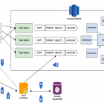
Amazon Redshift best practices suggest the use of the COPY command to perform data loads. This API operation uses all compute nodes in the cluster to load data in parallel, from sources such as Amazon S3, Amazon DynamoDB, Amazon EMR HDFS file systems, or any SSH connection.

When performing data loads, you should compress the files to be loaded whenever possible; Amazon Redshift supports both GZIP and LZO compression. It is more efficient to load a large number of small files than one large one, and the ideal file count is a multiple of the slice count. The number of slices per node depends on the node size of the cluster. By ensuring you have an equal number of files per slice, you can know that COPY execution will evenly use cluster resources and complete as quickly as possible.

The following query calculates statistics for each load:

SELECT a.tbl,
  trim(c.nspname) AS "schema", 
  trim(b.relname) AS "tablename", 
  sum(a.rows_inserted) AS "rows_inserted", 
  sum(d.distinct_files) AS files_scanned,  
  sum(d.MB_scanned) AS MB_scanned, 
  (sum(d.distinct_files)::numeric(19,3)/count(distinct a.query)::numeric(19,3))::numeric(19,3) AS avg_files_per_copy, 
  (sum(d.MB_scanned)/sum(d.distinct_files)::numeric(19,3))::numeric(19,3) AS avg_file_size_mb, 
  count(distinct a.query) no_of_copy, 
  max(a.query) AS sample_query, 
  (sum(d.MB_scanned)*1024*1000000/SUM(d.load_micro)) AS scan_rate_kbps, 
  (sum(a.rows_inserted)*1000000/SUM(a.insert_micro)) AS insert_rate_rows_ps 
FROM 
  (SELECT query, 
    tbl, 
    sum(rows) AS rows_inserted, 
    max(endtime) AS endtime, 
    datediff('microsecond',min(starttime),max(endtime)) AS insert_micro 
  FROM stl_insert 
  GROUP BY query, tbl) a,      
  pg_class b, 
  pg_namespace c,                 
  (SELECT b.query, 
    count(distinct b.bucket||b.key) AS distinct_files, 
    sum(b.transfer_size)/1024/1024 AS MB_scanned, 
    sum(b.transfer_time) AS load_micro 
  FROM stl_s3client b 
  WHERE b.http_method = 'GET' 
  GROUP BY b.query) d 
WHERE a.tbl = b.oid AND b.relnamespace = c.oid AND d.query = a.query 
GROUP BY 1,2,3 
ORDER BY 4 desc;

The following query shows the time taken to load a table, and the time taken to update the table statistics, both in seconds and as a percentage of the overall load process:

SELECT a.userid, 
  a.query, 
  round(b.comp_time::float/1000::float,2) comp_sec, 
  round(a.copy_time::float/1000::float,2) load_sec, 
  round(100*b.comp_time::float/(b.comp_time + a.copy_time)::float,2) ||'%' pct_complyze, 
  substring(q.querytxt,1,50) 
FROM (
  SELECT userid, 
    query, 
    xid, 
    datediff(ms,starttime,endtime) copy_time 
  FROM stl_query q 
  WHERE (querytxt ILIKE 'copy %from%') 
  AND exists (
    SELECT 1 
    FROM stl_commit_stats cs 
    WHERE cs.xid=q.xid) 
  AND exists (
    SELECT xid 
    FROM stl_query 
    WHERE query IN (
      SELECT distinct query 
      FROM stl_load_commits))) a 
LEFT JOIN (
  SELECT xid, 
    sum(datediff(ms,starttime,endtime)) comp_time 
  FROM stl_query q 
  WHERE (querytxt LIKE 'COPY ANALYZE %' OR querytxt LIKE 'analyze compression phase %') 
  AND exists (
    SELECT 1 
    FROM stl_commit_stats cs 
    WHERE cs.xid=q.xid) 
  AND exists (
    SELECT xid 
    FROM stl_query 
    WHERE query IN (
      SELECT distinct query 
      FROM stl_load_commits)) 
  GROUP BY 1) b 
ON b.xid = a.xid 
JOIN stl_query q 
ON q.query = a.query 
WHERE (b.comp_time IS NOT null) 
ORDER BY 6,5;

An anti-pattern is to insert data directly into Amazon Redshift, with single record inserts or the use of a multi-value INSERT statement, which allows up to 16 MB of data to be inserted at one time. These are leader node–based operations, and can create significant performance bottlenecks by maxing out the leader node network as data is distributed by the leader to the compute nodes.

Issue #10 – Inefficient use of Temporary Tables

Amazon Redshift provides temporary tables, which are like normal tables except that they are only visible within a single session. When the user disconnects the session, the tables are automatically deleted. Temporary tables can be created using the CREATE TEMPORARY TABLE syntax, or by issuing a SELECT … INTO #TEMP_TABLE query. The CREATE TABLE statement gives you complete control over the definition of the temporary table, while the SELECT … INTO and C(T)TAS commands use the input data to determine column names, sizes and data types, and use default storage properties.

These default storage properties may cause issues if not carefully considered. Amazon Redshift’s default table structure is to use EVEN distribution with no column encoding. This is a sub-optimal data structure for many types of queries, and if you are using the SELECT…INTO syntax you cannot set the column encoding or distribution and sort keys. If you use the CREATE TABLE AS (CTAS) syntax, you can specify a distribution style and sort keys, and Redshift will automatically apply LZO encoding for everything other than sort keys, booleans, reals and doubles. If you consider this automatic encoding sub-optimal, and require further control, use the CREATE TABLE syntax rather than CTAS.

If you are creating temporary tables, it is highly recommended that you convert all SELECT…INTO syntax to use the CREATE statement. This ensures that your temporary tables have column encodings and are distributed in a fashion that is sympathetic to the other entities that are part of the workflow. To perform a conversion of a statement which uses:

SELECT column_a, column_b INTO #my_temp_table FROM my_table;

You would analyse the temporary table for optimal column encoding:

And then convert the select/into statement to:

BEGIN;
CREATE TEMPORARY TABLE my_temp_table(
column_a varchar(128) encode lzo,
column_b char(4) encode bytedict)
distkey (column_a) -- Assuming you intend to join this table on column_a
sortkey (column_b); -- Assuming you are sorting or grouping by column_b
 
INSERT INTO my_temp_table SELECT column_a, column_b FROM my_table;
COMMIT;

You may also wish to analyze statistics on the temporary table, if it is used as a join table for subsequent queries:

ANALYZE my_temp_table;

This way, you retain the functionality of using temporary tables but control data placement on the cluster through distribution key assignment, and take advantage of the columnar nature of Amazon Redshift through use of column encoding.

Tip: Using explain plan alerts

The last tip is to use diagnostic information from the cluster during query execution. This is stored in an extremely useful view called STL_ALERT_EVENT_LOG. Use the perf_alert.sql admin script to diagnose issues that the cluster has encountered over the last seven days. This is an invaluable resource in understanding how your cluster develops over time.

Summary

Amazon Redshift is a powerful, fully managed data warehouse that can offer significantly increased performance and lower cost in the cloud. While Amazon Redshift can run any type of data model, you can avoid possible pitfalls that might decrease performance or increase cost, by being aware of how data is stored and managed. Run a simple set of diagnostic queries for common issues and ensure that you get the best performance possible.

If you have questions or suggestions, please leave a comment below.

Updated November 28, 2016

Related