
Elasticsearch之聚合aggregations
聚合可以讓我們極其方便的實現對資料的統計、分析。例如:
- 什麼品牌的手機最受歡迎?
- 這些手機的平均價格、最高價格、最低價格?
- 這些手機每月的銷售情況如何?
實現這些統計功能的比資料庫的sql要方便的多,而且查詢速度非常快,可以實現實時搜尋效果。
1 基本概念
Elasticsearch中的聚合,包含多種型別,最常用的兩種,一個叫桶,一個叫度量:
桶(bucket)
桶的作用,是按照某種方式對資料進行分組,每一組資料在ES中稱為一個桶,例如我們根據國籍對人劃分,可以得到中國桶、英國桶,日本桶……或者我們按照年齡段對人進行劃分:010,10
Elasticsearch中提供的劃分桶的方式有很多:
- Date Histogram Aggregation:根據日期階梯分組,例如給定階梯為周,會自動每週分為一組
- Histogram Aggregation:根據數值階梯分組,與日期類似
- Terms Aggregation:根據詞條內容分組,詞條內容完全匹配的為一組
- Range Aggregation:數值和日期的範圍分組,指定開始和結束,然後按段分組
- ……
綜上所述,我們發現bucket aggregations 只負責對資料進行分組,並不進行計算,因此往往bucket中往往會巢狀另一種聚合:metrics aggregations即度量
度量(metrics)
分組完成以後,我們一般會對組中的資料進行聚合運算,例如求平均值、最大、最小、求和等,這些在ES中稱為度量
比較常用的一些度量聚合方式:
- Avg Aggregation:求平均值
- Max Aggregation:求最大值
- Min Aggregation:求最小值
- Percentiles Aggregation:求百分比
- Stats Aggregation:同時返回avg、max、min、sum、count等
- Sum Aggregation:求和
- Top hits Aggregation:求前幾
- Value Count Aggregation:求總數
- ……
為了測試聚合,我們先批量匯入一些資料
建立索引:
PUT /cars
{
  "settings": {
    "number_of_shards": 1,
    "number_of_replicas": 0
  },
  "mappings": {
    "transactions": {
      "properties": {
        "color": {
          "type": "keyword"
        },
        "make": {
          "type": "keyword"
        }
      }
    }
  }
}
注意:在ES中,需要進行聚合、排序、過濾的欄位其處理方式比較特殊,因此不能被分詞。這裡我們將color和make這兩個文字型別的欄位設定為keyword型別,這個型別不會被分詞,將來就可以參與聚合
匯入資料
POST /cars/transactions/_bulk
{ "index": {}}
{ "price" : 10000, "color" : "red", "make" : "honda", "sold" : "2014-10-28" }
{ "index": {}}
{ "price" : 20000, "color" : "red", "make" : "honda", "sold" : "2014-11-05" }
{ "index": {}}
{ "price" : 30000, "color" : "green", "make" : "ford", "sold" : "2014-05-18" }
{ "index": {}}
{ "price" : 15000, "color" : "blue", "make" : "toyota", "sold" : "2014-07-02" }
{ "index": {}}
{ "price" : 12000, "color" : "green", "make" : "toyota", "sold" : "2014-08-19" }
{ "index": {}}
{ "price" : 20000, "color" : "red", "make" : "honda", "sold" : "2014-11-05" }
{ "index": {}}
{ "price" : 80000, "color" : "red", "make" : "bmw", "sold" : "2014-01-01" }
{ "index": {}}
{ "price" : 25000, "color" : "blue", "make" : "ford", "sold" : "2014-02-12" }
2 聚合為桶
首先,我們按照 汽車的顏色color來劃分桶
GET /cars/_search
{
    "size" : 0,
    "aggs" : {
        "popular_colors" : {
            "terms" : {
              "field" : "color"
            }
        }
    }
}
- size: 查詢條數,這裡設定為0,因為我們不關心搜尋到的資料,只關心聚合結果,提高效率
- aggs:宣告這是一個聚合查詢,是aggregations的縮寫
- popular_colors:給這次聚合起一個名字,任意。
- terms:劃分桶的方式,這裡是根據詞條劃分
- field:劃分桶的欄位
- terms:劃分桶的方式,這裡是根據詞條劃分
- popular_colors:給這次聚合起一個名字,任意。
結果:
{
  "took": 1,
  "timed_out": false,
  "_shards": {
    "total": 1,
    "successful": 1,
    "skipped": 0,
    "failed": 0
  },
  "hits": {
    "total": 8,
    "max_score": 0,
    "hits": []
  },
  "aggregations": {
    "popular_colors": {
      "doc_count_error_upper_bound": 0,
      "sum_other_doc_count": 0,
      "buckets": [
        {
          "key": "red",
          "doc_count": 4
        },
        {
          "key": "blue",
          "doc_count": 2
        },
        {
          "key": "green",
          "doc_count": 2
        }
      ]
    }
  }
}
- hits:查詢結果為空,因為我們設定了size為0
- aggregations:聚合的結果
- popular_colors:我們定義的聚合名稱
- buckets:查詢到的桶,每個不同的color欄位值都會形成一個桶
- key:這個桶對應的color欄位的值
- doc_count:這個桶中的文件數量
通過聚合的結果我們發現,目前紅色的小車比較暢銷!
3 桶內度量
前面的例子告訴我們每個桶裡面的文件數量,這很有用。 但通常,我們的應用需要提供更復雜的文件度量。 例如,每種顏色汽車的平均價格是多少?
因此,我們需要告訴Elasticsearch使用哪個欄位,使用何種度量方式進行運算,這些資訊要巢狀在桶內,度量的運算會基於桶內的文件進行
現在,我們為剛剛的聚合結果新增 求價格平均值的度量:
GET /cars/_search
{
    "size" : 0,
    "aggs" : {
        "popular_colors" : {
            "terms" : {
              "field" : "color"
            },
            "aggs":{
                "avg_price": {
                   "avg": {
                      "field": "price"
                   }
                }
            }
        }
    }
}
- aggs:我們在上一個aggs(popular_colors)中新增新的aggs。可見
度量也是一個聚合,度量是在桶內的聚合 - avg_price:聚合的名稱
- avg:度量的型別,這裡是求平均值
- field:度量運算的欄位
結果:
...
  "aggregations": {
    "popular_colors": {
      "doc_count_error_upper_bound": 0,
      "sum_other_doc_count": 0,
      "buckets": [
        {
          "key": "red",
          "doc_count": 4,
          "avg_price": {
            "value": 32500
          }
        },
        {
          "key": "blue",
          "doc_count": 2,
          "avg_price": {
            "value": 20000
          }
        },
        {
          "key": "green",
          "doc_count": 2,
          "avg_price": {
            "value": 21000
          }
        }
      ]
    }
  }
...
可以看到每個桶中都有自己的avg_price欄位,這是度量聚合的結果
4 桶內巢狀桶
剛剛的案例中,我們在桶內巢狀度量運算。事實上桶不僅可以巢狀運算, 還可以再巢狀其它桶。也就是說在每個分組中,再分更多組。
比如:我們想統計每種顏色的汽車中,分別屬於哪個製造商,按照make欄位再進行分桶
GET /cars/_search
{
    "size" : 0,
    "aggs" : {
        "popular_colors" : {
            "terms" : {
              "field" : "color"
            },
            "aggs":{
                "avg_price": {
                   "avg": {
                      "field": "price"
                   }
                },
                "maker":{
                    "terms":{
                        "field":"make"
                    }
                }
            }
        }
    }
}
- 原來的color桶和avg計算我們不變
- maker:在巢狀的aggs下新添一個桶,叫做maker
- terms:桶的劃分型別依然是詞條
- filed:這裡根據make欄位進行劃分
部分結果:
...
{"aggregations": {
    "popular_colors": {
      "doc_count_error_upper_bound": 0,
      "sum_other_doc_count": 0,
      "buckets": [
        {
          "key": "red",
          "doc_count": 4,
          "maker": {
            "doc_count_error_upper_bound": 0,
            "sum_other_doc_count": 0,
            "buckets": [
              {
                "key": "honda",
                "doc_count": 3
              },
              {
                "key": "bmw",
                "doc_count": 1
              }
            ]
          },
          "avg_price": {
            "value": 32500
          }
        },
        {
          "key": "blue",
          "doc_count": 2,
          "maker": {
            "doc_count_error_upper_bound": 0,
            "sum_other_doc_count": 0,
            "buckets": [
              {
                "key": "ford",
                "doc_count": 1
              },
              {
                "key": "toyota",
                "doc_count": 1
              }
            ]
          },
          "avg_price": {
            "value": 20000
          }
        },
        {
          "key": "green",
          "doc_count": 2,
          "maker": {
            "doc_count_error_upper_bound": 0,
            "sum_other_doc_count": 0,
            "buckets": [
              {
                "key": "ford",
                "doc_count": 1
              },
              {
                "key": "toyota",
                "doc_count": 1
              }
            ]
          },
          "avg_price": {
            "value": 21000
          }
        }
      ]
    }
  }
}
...
- 我們可以看到,新的聚合
maker被巢狀在原來每一個color的桶中。 - 每個顏色下面都根據
make欄位進行了分組 - 我們能讀取到的資訊:
- 紅色車共有4輛
- 紅色車的平均售價是 $32,500 美元。
- 其中3輛是 Honda 本田製造,1輛是 BMW 寶馬製造。
5.劃分桶的其它方式
前面講了,劃分桶的方式有很多,例如:
- Date Histogram Aggregation:根據日期階梯分組,例如給定階梯為周,會自動每週分為一組
- Histogram Aggregation:根據數值階梯分組,與日期類似
- Terms Aggregation:根據詞條內容分組,詞條內容完全匹配的為一組
- Range Aggregation:數值和日期的範圍分組,指定開始和結束,然後按段分組
剛剛的案例中,我們採用的是Terms Aggregation,即根據詞條劃分桶。
接下來,我們再學習幾個比較實用的:
5.1.階梯分桶Histogram
原理:
histogram是把數值型別的欄位,按照一定的階梯大小進行分組。你需要指定一個階梯值(interval)來劃分階梯大小。
舉例:
比如你有價格欄位,如果你設定interval的值為200,那麼階梯就會是這樣的:
0,200,400,600,…
上面列出的是每個階梯的key,也是區間的啟點。
如果一件商品的價格是450,會落入哪個階梯區間呢?計算公式如下:
bucket_key = Math.floor((value - offset) / interval) * interval + offset
value:就是當前資料的值,本例中是450
offset:起始偏移量,預設為0
interval:階梯間隔,比如200
因此你得到的key = Math.floor((450 - 0) / 200) * 200 + 0 = 400
操作一下:
比如,我們對汽車的價格進行分組,指定間隔interval為5000:
GET /cars/_search
{
  "size":0,
  "aggs":{
    "price":{
      "histogram": {
        "field": "price",
        "interval": 5000
      }
    }
  }
}
結果:
{
  "took": 21,
  "timed_out": false,
  "_shards": {
    "total": 5,
    "successful": 5,
    "skipped": 0,
    "failed": 0
  },
  "hits": {
    "total": 8,
    "max_score": 0,
    "hits": []
  },
  "aggregations": {
    "price": {
      "buckets": [
        {
          "key": 10000,
          "doc_count": 2
        },
        {
          "key": 15000,
          "doc_count": 1
        },
        {
          "key": 20000,
          "doc_count": 2
        },
        {
          "key": 25000,
          "doc_count": 1
        },
        {
          "key": 30000,
          "doc_count": 1
        },
        {
          "key": 35000,
          "doc_count": 0
        },
        {
          "key": 40000,
          "doc_count": 0
        },
        {
          "key": 45000,
          "doc_count": 0
        },
        {
          "key": 50000,
          "doc_count": 0
        },
        {
          "key": 55000,
          "doc_count": 0
        },
        {
          "key": 60000,
          "doc_count": 0
        },
        {
          "key": 65000,
          "doc_count": 0
        },
        {
          "key": 70000,
          "doc_count": 0
        },
        {
          "key": 75000,
          "doc_count": 0
        },
        {
          "key": 80000,
          "doc_count": 1
        }
      ]
    }
  }
}
你會發現,中間有大量的文件數量為0 的桶,看起來很醜。
我們可以增加一個引數min_doc_count為1,來約束最少文件數量為1,這樣文件數量為0的桶會被過濾
示例:
GET /cars/_search
{
  "size":0,
  "aggs":{
    "price":{
      "histogram": {
        "field": "price",
        "interval": 5000,
        "min_doc_count": 1
      }
    }
  }
}
結果:
{
  "took": 15,
  "timed_out": false,
  "_shards": {
    "total": 5,
    "successful": 5,
    "skipped": 0,
    "failed": 0
  },
  "hits": {
    "total": 8,
    "max_score": 0,
    "hits": []
  },
  "aggregations": {
    "price": {
      "buckets": [
        {
          "key": 10000,
          "doc_count": 2
        },
        {
          "key": 15000,
          "doc_count": 1
        },
        {
          "key": 20000,
          "doc_count": 2
        },
        {
          "key": 25000,
          "doc_count": 1
        },
        {
          "key": 30000,
          "doc_count": 1
        },
        {
          "key": 80000,
          "doc_count": 1
        }
      ]
    }
  }
}
完美,!
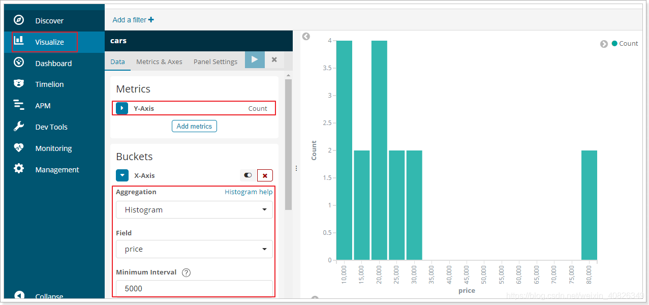
如果你用kibana將結果變為柱形圖,會更好看:
5.2.範圍分桶range
範圍分桶與階梯分桶類似,也是把數字按照階段進行分組,只不過range方式需要你自己指定每一組的起始和結束大小。