1.什麼是稀疏表示：

            假設我們用一個M*N的矩陣表示資料集X，每一行代表一個樣本，每一列代表樣本的一個屬性，一般而言，該矩陣是稠密的，即大多數元素不為0。 稀疏表示的含義是，尋找一個係數矩陣A（K*N）以及一個字典矩陣B（M*K），使得B*A儘可能的還原X，且A儘可能的稀疏。A便是X的稀疏表示。

        南大周志華老師寫的《機器學習》這本書上原文：“為普通稠密表達的樣本找到合適的字典，將樣本轉化為合適的稀疏表達形式，從而使學習任務得以簡化，模型複雜度得以降低，通常稱為‘字典學習’（dictionary learning），亦稱‘稀疏編碼’（sparse coding）”塊內容。

        表達為優化問題的話，字典學習的最簡單形式為： 

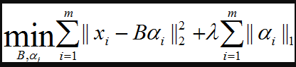
其中xi為第i個樣本，B為字典矩陣，aphai為xi的稀疏表示，lambda為大於0引數。 

      上式中第一個累加項說明了字典學習的第一個目標是字典矩陣與稀疏表示的線性組合儘可能的還原樣本；第二個累加項說明了alphai應該儘可能的稀疏。之所以用L1正規化是因為L1正規化正則化更容易獲得稀疏解。具體原因參看該書11.4章或移步機器學習中的範數規則化之（一）L0、L1與L2範數。字典學習便是學習出滿足上述最優化問題的字典B以及樣本的稀疏表示A（A{alpha1，alpha2，…，alphai}）。

2.字典學習：

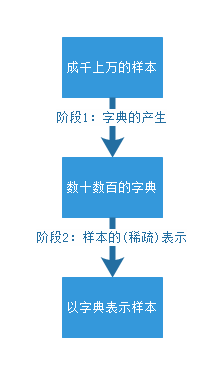
       該演算法理論包含兩個階段：字典構建階段（Dictionary Generate）和利用字典（稀疏的）表示樣本階段（Sparse coding with a precomputed dictionary）。這兩個階段（如下圖）的每個階段都有許多不同演算法可供選擇，每種演算法的誕生時間都不一樣，以至於稀疏字典學習的理論提出者已變得不可考。筆者嘗試找了Wikipedia和Google Scolar都無法找到這一系列理論的最早發起人。

出處：http://www.mamicode.com/info-detail-1568956.html

        字典學習的第一個好處——它實質上是對於龐大資料集的一種降維表示。第二，正如同字是句子最質樸的特徵一樣，字典學習總是嘗試學習蘊藏在樣本背後最質樸的特徵（假如樣本最質樸的特徵就是樣本最好的特徵）.稀疏表示的本質：用盡可能少的資源表示儘可能多的知識，這種表示還能帶來一個附加的好處，即計算速度快。我們希望字典裡的字可以盡能的少，但是卻可以儘可能的表示最多的句子。這樣的字典最容易滿足稀疏條件。也就是說，這個“字典”是這個“稀疏”私人訂製的。

第二部分 稀疏字典學習的Python實現

用Python實現稀疏字典學習需要三個前提條件

1.安裝NumPy

2.安裝SciPy

3.安裝Python機器學習工具包sklearn

為了避免過於麻煩的安裝，這裡我乾脆建議諸位讀者安裝Python的商業發行版Anaconda，內含python整合開發環境和數百個常用的python支援包。具體安裝過程和使用細節參見我的部落格附錄D Python介面大法。

樣例一：圖片的稀疏字典學習

這段程式碼來源於Python的Dictionary Learning的官方文獻教材，主要用途是教會使用者通過字典學習對圖片進行濾波處理。

step1：首先是各種工具包的匯入和測試樣例的匯入

from time import time

import matplotlib.pyplot as plt
import numpy as np
import scipy as sp

from sklearn.decomposition import MiniBatchDictionaryLearning
from sklearn.feature_extraction.image import extract_patches_2d
from sklearn.feature_extraction.image import reconstruct_from_patches_2d
from sklearn.utils.testing import SkipTest
from sklearn.utils.fixes import sp_version

if sp_version < (0, 12):
    raise SkipTest("Skipping because SciPy version earlier than 0.12.0 and "
                   "thus does not include the scipy.misc.face() image.")
try:
    from scipy import misc
    face = misc.face(gray=True)
except AttributeError:
    # Old versions of scipy have face in the top level package
    face = sp.face(gray=True)

第1行：匯入time模組，用於測算一些步驟的時間消耗

第3~5行：匯入Python科學計算的基本需求模組，主要包括NumPy（矩陣計算模組）、SciPy（科學計算模組）和matplotlib.pyplot模組（畫圖）。有了這三個模組，Python儼然已是基礎版的Matlab。

第7~11行：匯入稀疏字典學習所需要的函式，下面分行解釋

第7行：匯入MiniBatchDictionaryLearning，MiniBatch是字典學習的一種方法，這種方法專門應用於大資料情況下字典學習。當資料量非常大時，嚴格對待每一個樣本就會消耗大量的時間，而MiniBatch通過降低計算精度來換取時間利益，但是仍然能夠通過大量的資料學到合理的詞典。換言之，普通的DictionaryLearning做的是精品店，量少而精，但是價格高。MiniBatchDictionaryLearning做的是批發市場，量大不精，薄利多銷。

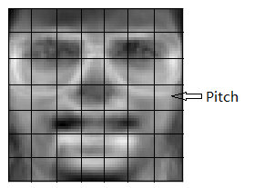
第8行：匯入碎片提取函式extract_patches_2d。呼叫該函式將一張圖片切割為一個一個的patch。如果一張圖片相當於一篇文章的話，那麼該函式的目標就是把文章中的每個句子都找到，這樣才方便提取蘊藏在每個句子中的字。圖片和patch的關係如下圖所示：

第9行：匯入圖片復原函式reconstruct_from_patches_2d，它可以通過patch復原一整張圖片。

第10行：匯入測試工具nose下的異常丟擲函式SkipTest

第11行：匯入SciPy版本檢測函式sp_version用於檢測版本高低，版本低於0.12的SciPy沒有我們需要的樣本測試用例

第13~15行：檢測SciPy版本，如果版本太低就丟擲一個異常。程式執行結束

第16~21行：嘗試開啟樣本測試用例，如果打不開就丟擲一個異常。

step2：通過測試樣例計算字典V

# Convert from uint8 representation with values between 0 and 255 to
# a floating point representation with values between 0 and 1.
face = face / 255.0

# downsample for higher speed
face = face[::2, ::2] + face[1::2, ::2] + face[::2, 1::2] + face[1::2, 1::2]
face = face / 4.0
height, width = face.shape

# Distort the right half of the image
print(‘Distorting image...‘)
distorted = face.copy()
distorted[:, width // 2:] += 0.075 * np.random.randn(height, width // 2)

# Extract all reference patches from the left half of the image
print(‘Extracting reference patches...‘)
t0 = time()
patch_size = (7, 7)
data = extract_patches_2d(distorted[:, :width // 2], patch_size)
data = data.reshape(data.shape[0], -1)
data -= np.mean(data, axis=0)
data /= np.std(data, axis=0)
print(‘done in %.2fs.‘ % (time() - t0))
print(‘Learning the dictionary...‘)
t0 = time()
dico = MiniBatchDictionaryLearning(n_components=100, alpha=1, n_iter=500)
V = dico.fit(data).components_
dt = time() - t0
print(‘done in %.2fs.‘ % dt)

plt.figure(figsize=(4.2, 4))
for i, comp in enumerate(V[:100]):
    plt.subplot(10, 10, i + 1)
    plt.imshow(comp.reshape(patch_size), cmap=plt.cm.gray_r,
               interpolation=‘nearest‘)
    plt.xticks(())
    plt.yticks(())
plt.suptitle(‘Dictionary learned from face patches\n‘ +
             ‘Train time %.1fs on %d patches‘ % (dt, len(data)),
             fontsize=16)
plt.subplots_adjust(0.08, 0.02, 0.92, 0.85, 0.08, 0.23)#left, right, bottom, top, wspace, hspace

第3行：讀入的face大小在0~255之間，所以通過除以255將face的大小對映到0~1上去

第6~7行：對圖形進行取樣，把圖片的長和寬各縮小一般。記住array矩陣的訪問方式      array[起始點：終結點（不包括）：步長]

第8行：圖片的長寬大小

第12行：將face的內容複製給distorted，這裡不用等號因為等號在python中其實是地址的引用。

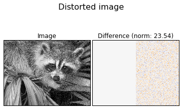
第13行：對照片的右半部分加上噪聲，之所以左半部分不加是因為教材想要產生一個對比的效果

第17行：開始計時，並儲存在t0中

第18行：tuple格式的pitch大小

第19行：對圖片的左半部分（未加噪聲的部分）提取pitch

第20行：用reshape函式對data(94500,7,7)進行整形，reshape中如果某一位是-1，則這一維會根據（元素個數/已指明的維度）來計算這裡經過整形後data變成（94500，49）

第21~22行：每一行的data減去均值除以方差，這是zscore標準化的方法

第26行：初始化MiniBatchDictionaryLearning類，並按照初始引數初始化類的屬性

第27行：呼叫fit方法對傳入的樣本集data進行字典提取，components_返回該類fit方法的運算結果，也就是我們想要的字典V

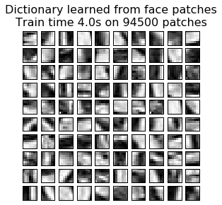
第31~41行：畫出V中的字典，下面逐行解釋

第31行：figsize方法指明圖片的大小，4.2英寸寬，4英寸高。其中一英寸的定義是80個畫素點

第32行：迴圈畫出100個字典V中的字

第41行：6個引數與註釋後的6個屬性對應

執行程式，檢視輸出結果：

step3：畫出標準影象和真正的噪聲，方便同之後字典學習學到的噪聲相比較

def show_with_diff(image, reference, title):
    """Helper function to display denoising"""
    plt.figure(figsize=(5, 3.3))
    plt.subplot(1, 2, 1)
    plt.title(‘Image‘)
    plt.imshow(image, vmin=0, vmax=1, cmap=plt.cm.gray,
               interpolation=‘nearest‘)
    plt.xticks(())
    plt.yticks(())
    plt.subplot(1, 2, 2)
    difference = image - reference

    plt.title(‘Difference (norm: %.2f)‘ % np.sqrt(np.sum(difference ** 2)))
    plt.imshow(difference, vmin=-0.5, vmax=0.5, cmap=plt.cm.PuOr,
               interpolation=‘nearest‘)
    plt.xticks(())
    plt.yticks(())
    plt.suptitle(title, size=16)
    plt.subplots_adjust(0.02, 0.02, 0.98, 0.79, 0.02, 0.2)

show_with_diff(distorted, face, ‘Distorted image‘)

程式輸出如下圖所示：

step4：測試不同的字典學習方法和引數對字典學習的影響

print(‘Extracting noisy patches... ‘)
t0 = time()
data = extract_patches_2d(distorted[:, width // 2:], patch_size)
data = data.reshape(data.shape[0], -1)
intercept = np.mean(data, axis=0)
data -= intercept
print(‘done in %.2fs.‘ % (time() - t0))

transform_algorithms = [
    (‘Orthogonal Matching Pursuit\n1 atom‘, ‘omp‘,
     {‘transform_n_nonzero_coefs‘: 1}),
    (‘Orthogonal Matching Pursuit\n2 atoms‘, ‘omp‘,
     {‘transform_n_nonzero_coefs‘: 2}),
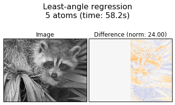
    (‘Least-angle regression\n5 atoms‘, ‘lars‘,
     {‘transform_n_nonzero_coefs‘: 5}),
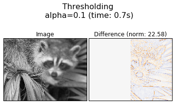
    (‘Thresholding\n alpha=0.1‘, ‘threshold‘, {‘transform_alpha‘: .1})]

reconstructions = {}
for title, transform_algorithm, kwargs in transform_algorithms:
    print(title + ‘...‘)
    reconstructions[title] = face.copy()
    t0 = time()
    dico.set_params(transform_algorithm=transform_algorithm, **kwargs)
    code = dico.transform(data)
    patches = np.dot(code, V)

    patches += intercept
    patches = patches.reshape(len(data), *patch_size)
    if transform_algorithm == ‘threshold‘:
        patches -= patches.min()
        patches /= patches.max()
    reconstructions[title][:, width // 2:] = reconstruct_from_patches_2d(
        patches, (height, width // 2))
    dt = time() - t0
    print(‘done in %.2fs.‘ % dt)
    show_with_diff(reconstructions[title], face,
                   title + ‘ (time: %.1fs)‘ % dt)

plt.show()

第3行：提取照片中被汙染過的右半部進行字典學習。

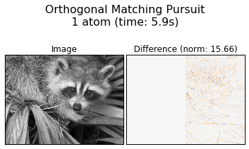
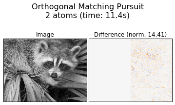
第10~16行：四中不同的字典表示策略

第23行：通過set_params對第二階段的引數進行設定

第24行：transform根據set_params對設完引數的模型進行字典表示，表示結果放在code中。code總共有100列，每一列對應著V中的一個字典元素，所謂稀疏性就是code中每一行的大部分元素都是0，這樣就可以用盡可能少的字典元素表示回去。

第25行：code矩陣乘V得到復原後的矩陣patches

第28行：將patches從（94500，49）變回（94500，7，7）

第32行：通過reconstruct_from_patches_2d函式將patches重新拼接回圖片

該程式輸出為四中不同轉換演算法下的降噪效果：

第二部分程式碼出處：

http://www.mamicode.com/info-detail-1568956.html