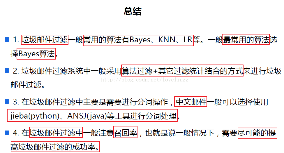
機器學習專案(一)——垃圾郵件的過濾技術
阿新 • • 發佈:2019-01-22
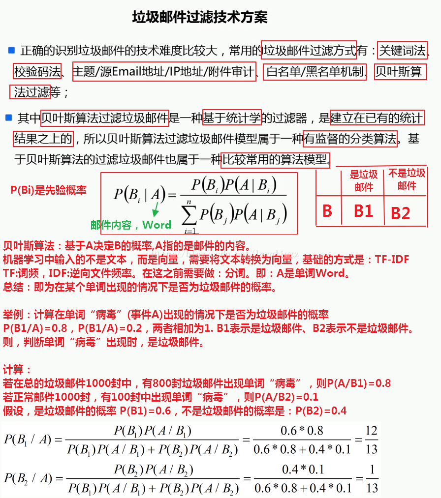
一、垃圾郵件過濾技術專案需求與設計方案


二、資料的內容分析
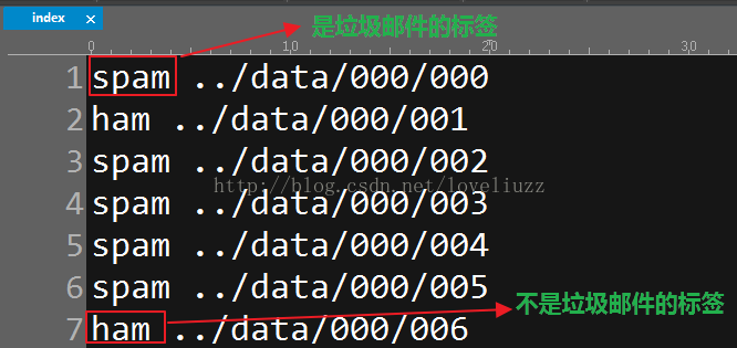
(1、是否為垃圾郵件的標籤,spam——是垃圾郵件;ham——不是垃圾郵件)
(2、郵件的內容分析——主要包含:發件人、收件人、發件時間以及郵件的內容)


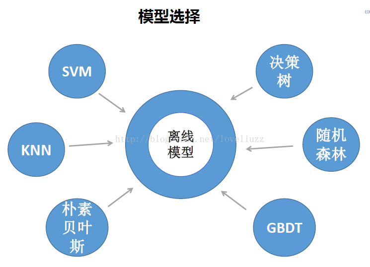
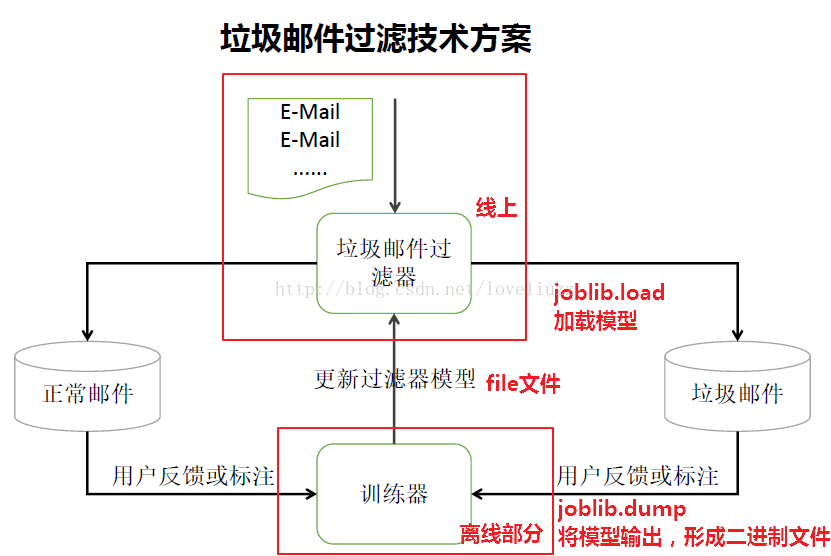
三、需求分析、模型選擇與架構

四、資料清洗
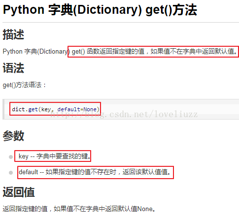
(一)·程式碼中應用的知識點
(1)字典的get()函式

(2)os.listdir()

(二)資料清洗程式碼
#!/usr/bin/env python
# -*- coding:utf-8 -*-
# Author:ZhengzhengLiu

import os

#1、索引檔案(分類標籤)讀取,該檔案中分為兩列
#第一列:分類標籤是否為垃圾郵件(是:spam、否:ham);
# 第二列:存放郵件對應資料夾路徑,兩列之間通過空格分割
def read_index_file(file_path):
    type_dict = {"spam":"1","ham":"0"}      #用字典存放垃圾郵件的分類標籤
    index_file = open(file_path)
    index_dict = {}
    try:
        for line in index_file:  # 按行迴圈讀取檔案
            arr = line.split(" ")  # 用“空格”進行分割
            #pd.read_csv("full/index",sep=" ")      #pandas來寫與上面等價
            if len(arr) == 2:       #分割完之後如果長度是2
                key,value = arr     ##分別將spam  ../data/178/129賦值給key與value
            #新增到欄位中
            value = value.replace("../data","").replace("\n","")    #替換
            # 字典賦值,字典名[鍵]=值,lower()將所有的字母轉換成小寫
            index_dict[value] = type_dict[key.lower()]      #
    finally:
        index_file.close()
    return index_dict

#2、郵件的檔案內容資料讀取
def read_file(file_path):
    # 讀操作,郵件資料編碼為"gb2312",資料讀取有異常就ignore忽略
    file = open(file_path,"r",encoding="gb2312",errors="ignore")
    content_dict = {}

    try:
        is_content = False
        for line in file:  # 按行讀取
            line = line.strip()  # 每行的空格去掉用strip()
            if line.startswith("From:"):
                content_dict["from"] = line[5:]
            elif line.startswith("To:"):
                content_dict["to"] = line[3:]
            elif line.startswith("Date:"):
                content_dict["data"] = line[5:]
            elif not line:
                # 郵件內容與上面資訊存在著第一個空行,遇到空行時,這裡標記為True以便進行下面的郵件內容處理
                # line檔案的行為空時是False,不為空時是True
                is_content = True

            # 處理郵件內容(處理到為空的行時接著處理郵件的內容)
            if is_content:
                if "content" in content_dict:
                    content_dict["content"] += line
                else:
                    content_dict["content"] = line
    finally:
        file.close()

    return content_dict

#3、郵件資料處理(內容的拼接,並用逗號進行分割)
def process_file(file_path):
    content_dict = read_file(file_path)

    #進行處理(拼接),get()函式返回指定鍵的值,指定鍵的值不存在用指定的預設值unkown代替
    result_str = content_dict.get("from","unkown").replace(",","").strip()+","
    result_str += content_dict.get("to","unkown").replace(",","").strip()+","
    result_str += content_dict.get("data","unkown").replace(",","").strip()+","
    result_str += content_dict.get("content","unkown").replace(",","").strip()
    return result_str

#4、開始進行資料處理——函式呼叫
## os.listdir    返回指定的資料夾包含的檔案或資料夾包含的名稱列表
index_dict = read_index_file('../data/full/index')
list0 = os.listdir('../data/data')      #list0是範圍為[000-215]的列表
# print(list0)
for l1 in list0:    # l1:迴圈000--215
    l1_path = '../data/data/' + l1      #l1_path   ../data/data/215
    print('開始處理資料夾:' + l1_path)
    list1 = os.listdir(l1_path)     #list1:['000', '001', '002', '003'....'299']
    # print(list1)
    write_file_path = '../data/process01_' + l1
    with open(write_file_path, "w", encoding='utf-8') as writer:
        for l2 in list1:  # l2:迴圈000--299
            l2_path = l1_path + "/" + l2  # l2_path   ../data/data/215/000
            # 得到具體的檔案內容後,進行檔案資料的讀取
            index_key = "/" + l1 + "/" + l2  # index_key:  /215/000

            if index_key in index_dict:
                # 讀取資料
                content_str = process_file(l2_path)
                # 新增分類標籤(0、1)也用逗號隔開
                content_str += "," + index_dict[index_key] + "\n"
                # 進行資料輸出
                writer.writelines(content_str)

# 再合併所有第一次構建好的內容
with open('../data/result_process01', 'w', encoding='utf-8') as writer:
    for l1 in list0:
        file_path = '../data/process01_' + l1
        print("開始合併檔案:" + file_path)

        with open(file_path, encoding='utf-8') as file:
            for line in file:
                writer.writelines(line)
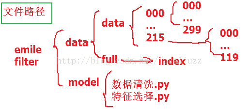
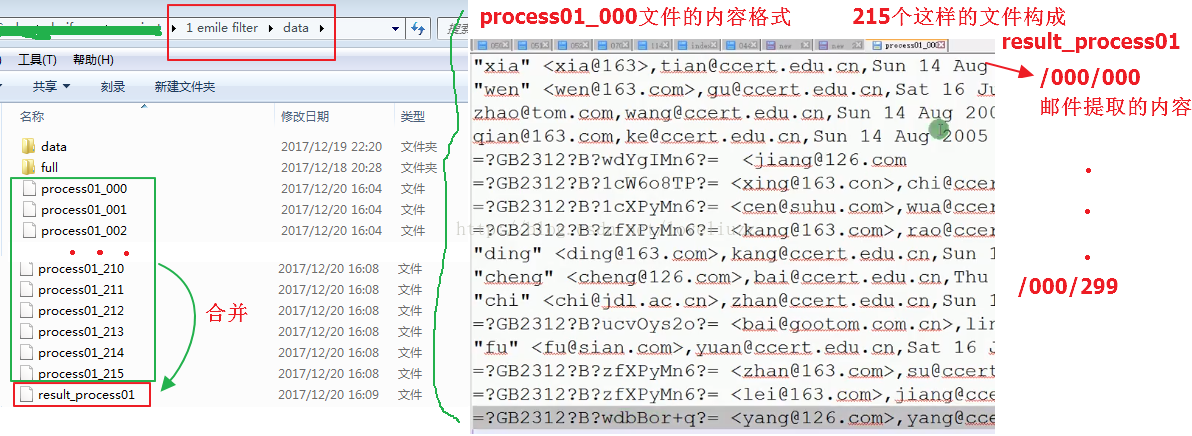
(三)郵件存放路徑框架與各步驟執行結果


最後執行的結果:

五、特徵工程
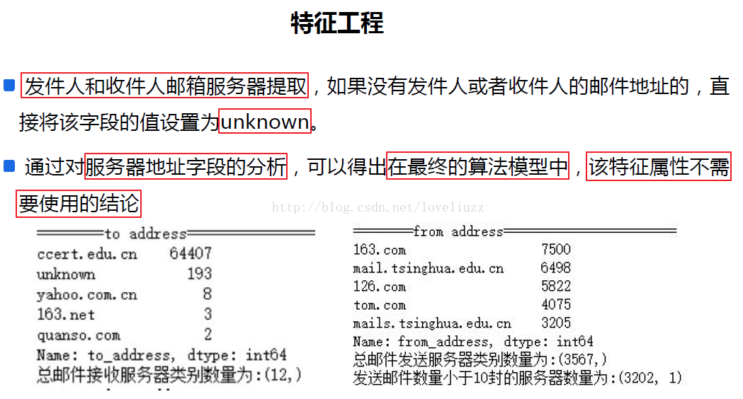
(一)郵件伺服器處理
知識點應用:


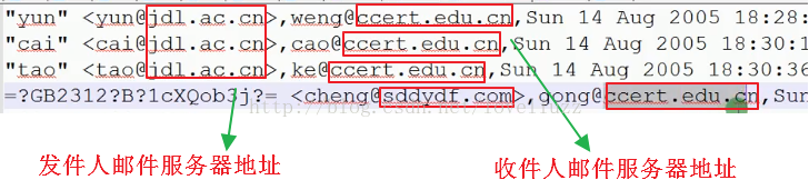
#!/usr/bin/env python
# -*- coding:utf-8 -*-
# Author:ZhengzhengLiu

import re
import time
import numpy as np
import pandas as pd
import matplotlib as mpl
import matplotlib.pyplot as plt

## 設定字符集,防止中文亂碼
mpl.rcParams['font.sans-serif']=[u'simHei']
mpl.rcParams['axes.unicode_minus']=False


# 1、檔案資料讀取
df = pd.read_csv("../data/result_process01",sep=",",header=None,
                 names=["from","to","date","content","label"])
# print(df.head())

#2(1)、特徵工程1 =>提取發件人和收件人的郵件伺服器地址
def extract_email_server_address(str1):
    it = re.findall(r"@([A-Za-z0-9]*\.[A-Za-z0-9\.]+)",str(str1))
    result = ""
    if len(it)>0:
        result = it[0]
    if not result:
        result = "unknown"
    return result

df["to_address"] = pd.Series(map(lambda str:extract_email_server_address(str),df["to"]))
df["from_address"] = pd.Series(map(lambda str:extract_email_server_address(str),df["from"]))
# print(df.head(2))

#2(2)、特徵工程1 =>檢視郵件伺服器的數量
print("=================to address================")
print(df.to_address.value_counts().head(5))
print("總郵件接收伺服器類別數量為:"+str(df.to_address.unique().shape))

print("=================from address================")
print(df.from_address.value_counts().head(5))
print("總郵件接收伺服器類別數量為:"+str(df.from_address.unique().shape))

from_address_df = df.from_address.value_counts().to_frame()
len_less_10_from_adderss_count = from_address_df[from_address_df.from_address<=10].shape
print("傳送郵件數量小於10封的伺服器數量為:"+str(len_less_10_from_adderss_count))
(二)時間屬性處理

#3、特徵工程2 =>郵件的時間提取
def extract_email_date(str1):
    if not isinstance(str1,str):  #判斷變數是否是str型別
        str1 = str(str1)    #str型別的強轉
    str_len = len(str1)

    week = ""
    hour = ""
    # 0表示:上午[8,12];1表示:下午[13,18];2表示:晚上[19,23];3表示:凌晨[0,7]
    time_quantum = ""

    if str_len < 10:
        #unknown
        week = "unknown"
        hour = "unknown"
        time_quantum ="unknown"
        pass
    elif str_len == 16:
        # 2005-9-2 上午10:55
        rex = r"(\d{2}):\d{2}"  # \d  匹配任意數字,這裡匹配10:55
        it = re.findall(rex,str1)
        if len(it) == 1:
            hour = it[0]
        else:
            hour = "unknown"
        week = "Fri"
        time_quantum = "0"
        pass
    elif str_len == 19:
        # Sep 23 2005 1:04 AM
        week = "Sep"
        hour = "01"
        time_quantum = "3"
        pass
    elif str_len == 21:
        # August 24 2005 5:00pm
        week = "Wed"
        hour = "17"
        time_quantum = "1"
        pass
    else:
        #匹配一個字元開頭,+表示至少一次  \d 表示數字   ?表示可有可無  *? 非貪婪模式
        rex = r"([A-Za-z]+\d?[A-Za-z]*) .*?(\d{2}):\d{2}:\d{2}.*"
        it = re.findall(rex,str1)
        if len(it) == 1 and len(it[0]) == 2:
            week = it[0][0][-3]
            hour = it[0][1]
            int_hour = int(hour)
            if int_hour < 8:
                time_quantum = "3"
            elif int_hour < 13:
                time_quantum = "0"
            elif int_hour < 19:
                time_quantum = "1"
            else:
                time_quantum = "2"
            pass
        else:
            week = "unknown"
            hour = "unknown"
            time_quantum = "unknown"
    week = week.lower()
    hour = hour.lower()
    time_quantum = time_quantum.lower()
    return (week,hour,time_quantum)

#資料轉換
data_time_extract_result = list(map(lambda st:extract_email_date(st),df["date"]))
df["date_week"] = pd.Series(map(lambda t:t[0],data_time_extract_result))
df["date_hour"] = pd.Series(map(lambda t:t[1],data_time_extract_result))
df["date_time_quantum"] = pd.Series(map(lambda t:t[2],data_time_extract_result))
print(df.head(2))

print("=======星期屬性欄位描述======")
print(df.date_week.value_counts().head(3))
print(df[["date_week","label"]].groupby(["date_week","label"])["label"].count())

print("=======小時屬性欄位描述======")
print(df.date_hour.value_counts().head(3))
print(df[['date_hour', 'label']].groupby(['date_hour', 'label'])['label'].count())

print("=======時間段屬性欄位描述======")
print(df.date_hour.value_counts().head(3))
print(df[["date_time_quantum","label"]].groupby(["date_time_quantum","label"])["label"].count())

#新增是否有時間
df["has_date"] = df.apply(lambda c: 0 if c["date_week"] == "unknown" else 1,axis=1)
print(df.head(2))

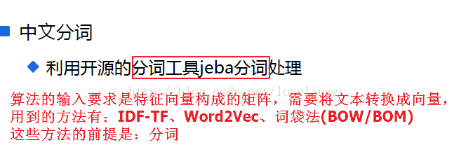
(三)郵件內容分詞——jieba分詞

#4、特徵工程之三 => jieba分詞操作
#將文字型別全部轉換為str型別,然後進行分詞操作
df["content"] = df["content"].astype("str")
'''
#1、jieba分詞的重點在於:自定義詞典
#2、jieba新增分詞字典,jieba.load_userdict("userdict.txt"),字典格式為:單詞 詞頻(可選的) 詞性(可選的)
# 詞典構建方式:一般都是基於jieba分詞之後的效果進行人工干預
#3、新增新詞、刪除詞 jieba.add_word("") jieba.del_word("")
#4、jieba.cut: def cut(self, sentence, cut_all=False, HMM=True)
# sentence:需要分割的文字,cut_all:分割模式,分為精準模式False、全分割True,HMM:新詞可進行推測
#5、長文字採用精準分割,短文字採用全分割模式
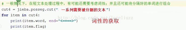
# 一般在短文字處理過程中還需要考慮詞性,並且還可能將分割好的單詞進行組合
# 詞性需要匯入的包:import jieba.posseg
'''
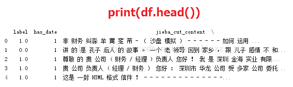
df["jieba_cut_content"] = list(map(lambda st:" ".join(jieba.cut(st)),df["content"])) #分開的詞用空格隔開
print(df.head(2))執行結果為:

注意內容:
(四)郵件資訊量/長度對是否為垃圾郵件的影響
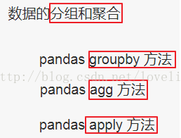
(1)應用知識點——groupby()技術
詳細參照連結:http://www.jianshu.com/p/2d49cb87626b
在資料分析中,我們往往需要在將資料拆分,在每一個特定的組裡進行運算。比如根據教育水平和年齡段計算某個城市的工作人口的平均收入。pandas中的groupby提供了一個高效的資料的分組運算。我們通過一個或者多個分類變數資料拆分,然後分別在拆分以後的資料上進行需要的計算。

#5、特徵工程之四 =>郵件長度對是否是垃圾郵件的影響
def process_content_length(lg):
    if lg < 10:
        return 0
    elif lg <= 100:
        return 1
    elif lg <= 500:
        return 2
    elif lg <= 1000:
        return 3
    elif lg <= 1500:
        return 4
    elif lg <= 2000:
        return 5
    elif lg <= 2500:
        return 6
    elif lg <= 3000:
        return 7
    elif lg <= 4000:
        return 8
    elif lg <= 5000:
        return 9
    elif lg <= 10000:
        return 10
    elif lg <= 20000:
        return 11
    elif lg <= 30000:
        return 12
    elif lg <= 50000:
        return 13
    else:
        return 14

df["content_length"] = pd.Series(map(lambda st:len(st),df["content"]))
df["content_length_type"] = pd.Series(map(lambda st:process_content_length(st),df["content_length"]))
#按照郵件長度類別和標籤進行分組groupby,抽取這兩列資料相同的放到一起,
# 用agg和內建函式count聚合不同長度郵件分貝是否為垃圾郵件的數量,
# reset_insex:將物件重新進行索引的構建
df2 = df.groupby(["content_length_type","label"])["label"].agg(["count"]).reset_index()
#label == 1:是垃圾郵件,對長度和數量進行重新命名,count命名為c1
df3 = df2[df2.label == 1][["content_length_type","count"]].rename(columns={"count":"c1"})
df4 = df2[df2.label == 0][["content_length_type","count"]].rename(columns={"count":"c2"})
df5 = pd.merge(df3,df4)  #資料集的合併,pandas.merge可依據一個或多個鍵將不同DataFrame中的行連線起來

df5["c1_rage"] = df5.apply(lambda r:r["c1"]/(r["c1"]+r["c2"]),axis=1)   #按行進行統計
df5["c2_rage"] = df5.apply(lambda r:r["c2"]/(r["c1"]+r["c2"]),axis=1)
print(df5.head())

#畫圖
plt.plot(df5["content_length_type"],df5["c1_rage"],label=u"垃圾郵件比例")
plt.plot(df5["content_length_type"],df5["c2_rage"],label=u"正常郵件比例")
plt.xlabel(u"郵件長度標記")
plt.ylabel(u"郵件比例")
plt.grid(True)
plt.legend(loc=0)
plt.savefig("垃圾和正常郵件比例.png")
plt.show()
執行結果:

(五)新增訊號量
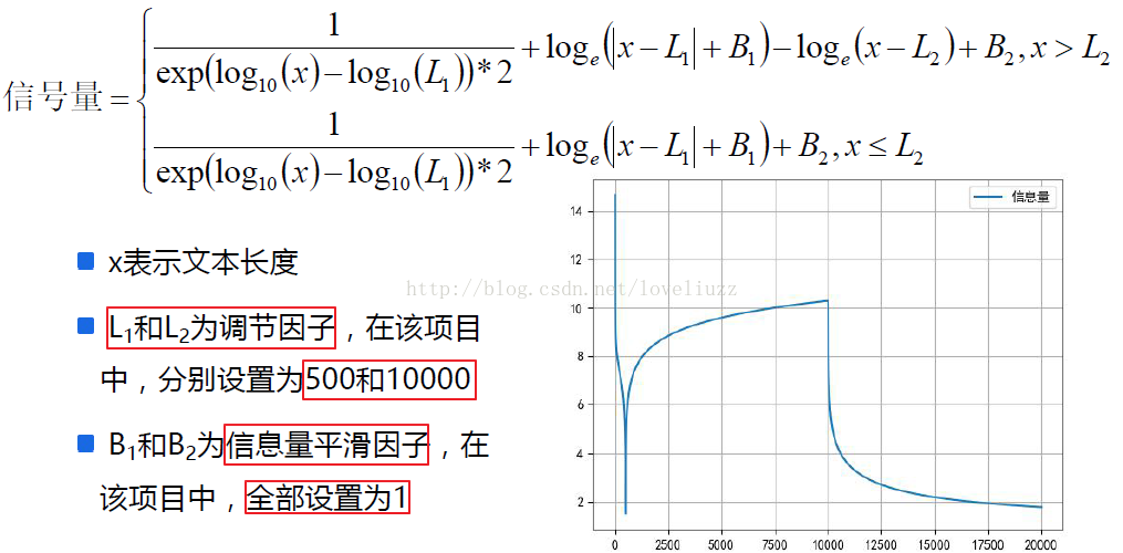
#6、特徵工程之五 ==> 新增訊號量
def precess_content_sema(x):
    if x>10000:
        return 0.5/np.exp(np.log10(x)-np.log10(500))+np.log(abs(x-500)+1)-np.log(abs(x-10000))+1
    else:
        return 0.5/np.exp(np.log10(x)-np.log10(500))+np.log(abs(x-500)+1)+1

a = np.arange(1,20000)
plt.plot(a,list(map(lambda t:precess_content_sema(t),a)),label=u"資訊量")
plt.grid(True)
plt.legend(loc=0)
plt.savefig("資訊量.png")
plt.show()

df["content_sema"] = list(map(lambda st:precess_content_sema(st),df["content_length"]))
print(df.head(2))
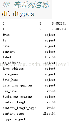
#檢視列名稱
print(df.dtypes)

#獲取需要的列,drop刪除不需要的列
df.drop(["from","to","date","content","to_address","from_address",
         "date_week","date_hour","date_time_quantum","content_length",
         "content_length_type"],1,inplace=True)
print(df.info())
print(df.head())

#結果輸出到CSV檔案中
df.to_csv("../data/result_process02",encoding="utf-8",index=False)
執行結果:


六、模型效果評估

#!/usr/bin/env python
# -*- coding:utf-8 -*-
# Author:ZhengzhengLiu
import time
import numpy as np
import pandas as pd
import matplotlib as mpl
import matplotlib.pyplot as plt
from sklearn.feature_extraction.text import CountVectorizer,TfidfVectorizer
from sklearn.model_selection import train_test_split
from sklearn.decomposition import TruncatedSVD #降維
from sklearn.naive_bayes import BernoulliNB #伯努利分佈的貝葉斯公式
from sklearn.metrics import f1_score,precision_score,recall_score
## 設定字符集,防止中文亂碼
mpl.rcParams['font.sans-serif']=[u'simHei']
mpl.rcParams['axes.unicode_minus']=False
#1、檔案資料讀取
df = pd.read_csv("../data/result_process02",encoding="utf-8",sep=",")
#如果有nan值,進行上刪除操作
df.dropna(axis=0,how="any",inplace=True) #刪除表中含有任何NaN的行
print(df.head())
print(df.info())
#2、資料分割
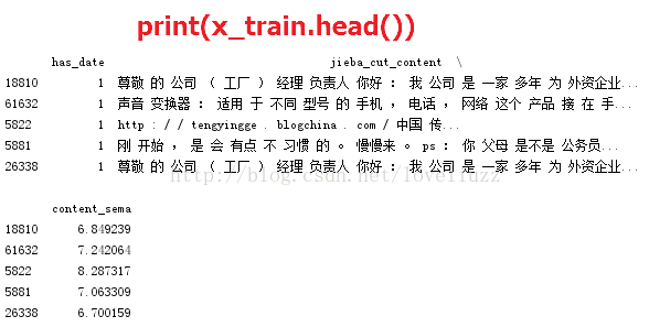
x_train,x_test,y_train,y_test = train_test_split(df[["has_date","jieba_cut_content","content_sema"]],
df["label"],test_size=0.2,random_state=0)
print("訓練資料集大小:%d" %x_train.shape[0])
print("測試資料集大小:%d" %x_test.shape[0])
print(x_train.head())
#3、開始模型訓練
#3.1、特徵工程,將文字資料轉換為數值型資料
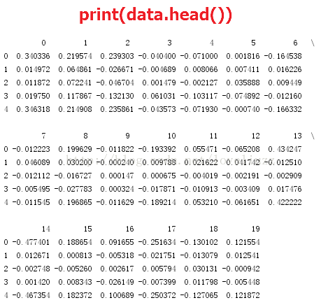
transformer = TfidfVectorizer(norm="l2",use_idf=True)
svd = TruncatedSVD(n_components=20) #奇異值分解,降維
jieba_cut_content = list(x_train["jieba_cut_content"].astype("str"))
transformer_model = transformer.fit(jieba_cut_content)
df1 = transformer_model.transform(jieba_cut_content)
svd_model = svd.fit(df1)
df2 = svd_model.transform(df1)
data = pd.DataFrame(df2)
print(data.head())
print(data.info())
#3.2、資料合併
data["has_date"] = list(x_train["has_date"])
data["content_sema"] = list(x_train["content_sema"])
print("========資料合併後的data資訊========")
print(data.head())
print(data.info())
t1 = time.time()
nb = BernoulliNB(alpha=1.0,binarize=0.0005) #貝葉斯分類模型構建
model = nb.fit(data,y_train)
t = time.time()-t1
print("貝葉斯模型構建時間為:%.5f ms" %(t*1000))
#4.1 對測試資料進行轉換
jieba_cut_content_test = list(x_test["jieba_cut_content"].astype("str"))
data_test = pd.DataFrame(svd_model.transform(transformer_model.transform(jieba_cut_content_test)))
data_test["has_date"] = list(x_test["has_date"])
data_test["content_sema"] = list(x_test["content_sema"])
print(data_test.head())
print(data_test.info())
#4.2 對測試資料進行測試
y_predict = model.predict(data_test)
#5、效果評估
print("準確率為:%.5f" % precision_score(y_test,y_predict))
print("召回率為:%.5f" % recall_score(y_test,y_predict))
print("F1值為:%.5f" % f1_score(y_test,y_predict))
執行結果: