python 實現案例

1、選取資料

 
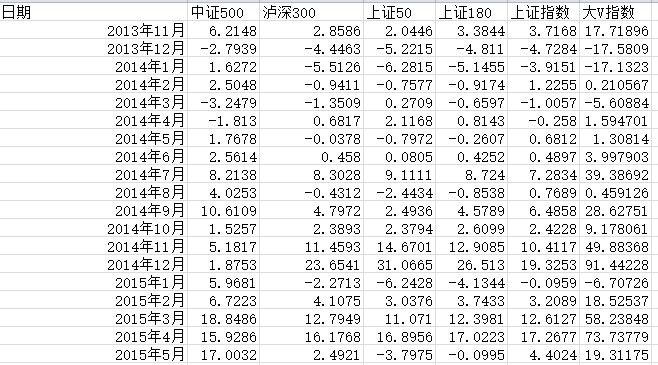
執行程式碼

#!usr/bin/env python
#_*_ coding:utf-8 _*_
import pandas as pd
import seaborn as sns
import matplotlib.pyplot as plt
import matplotlib as mpl   #顯示中文
def mul_lr():
    pd_data=pd.read_excel('C:\\Users\\lenovo\\Desktop\\test.xlsx')
    print('pd_data.head(10)=\n{}'.format(pd_data.head(10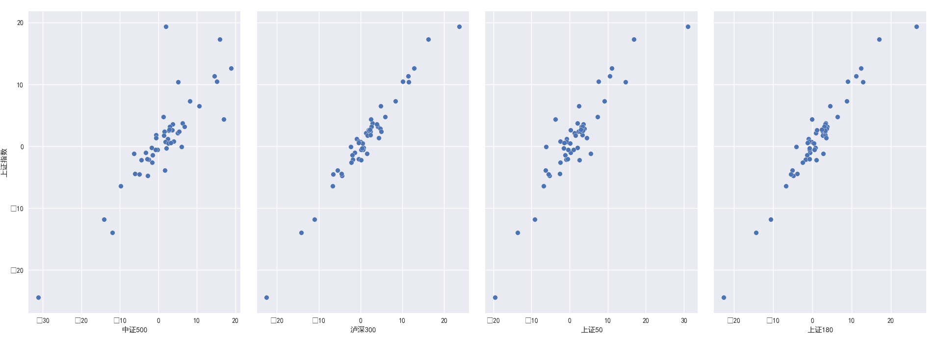
 
)))
mpl.rcParams['font.sans-serif'] = ['SimHei']  #配置顯示中文，否則亂碼
mpl.rcParams['axes.unicode_minus']=False #用來正常顯示負號，如果是plt畫圖，則將mlp換成plt
sns.pairplot(pd_data, x_vars=['中證500','瀘深300','上證50','上證180'], y_vars='上證指數',kind="reg", size=5, aspect=0.7)
plt.show()#注意必須加上這一句，否則無法顯示。

新增引數kind=”reg”結果，關於畫圖方面可[參考連線] 

#####2、構建訓練集與測試級，並構建模型

from sklearn.model_selection import train_test_split #這裡是引用了交叉驗證
from sklearn.linear_model import LinearRegression  #線性迴歸
from sklearn import metrics
import numpy as np
import matplotlib.pyplot as plt
def mul_lr():   #續前面程式碼
    #剔除日期資料，一般沒有這列可不執行，選取以下資料http://blog.csdn.net/chixujohnny/article/details/51095817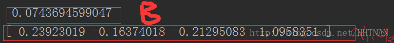
 

    X=pd_data.loc[:,('中證500','瀘深300','上證50','上證180')]
    y=pd_data.loc[:,'上證指數']
    X_train,X_test, y_train, y_test = train_test_split(X,y,test_size = 0.2,random_state=100)
    print ('X_train.shape={}\n y_train.shape ={}\n X_test.shape={}\n,  y_test.shape={}'.format(X_train.shape,y_train.shape, X_test.shape,y_test.shape))
    linreg = LinearRegression()
    model=linreg.fit(X_train, y_train)
    print (model)
    # 訓練後模型截距
    print (linreg.intercept_)
    # 訓練後模型權重（特徵個數無變化）
    print (linreg.coef_)

    feature_cols = ['中證500','瀘深300','上證50','上證180','上證指數']
    B=list(zip(feature_cols,linreg.coef_))
    print(B)

3、模型預測

    #預測
    y_pred = linreg.predict(X_test)
    print (y_pred) #10個變數的預測結果

4、模型評估

    #評價
    #(1) 評價測度
    # 對於分類問題，評價測度是準確率，但這種方法不適用於迴歸問題。我們使用針對連續數值的評價測度(evaluation metrics)。
    # 這裡介紹3種常用的針對線性迴歸的測度。
    # 1)平均絕對誤差(Mean Absolute Error, MAE)
    # (2)均方誤差(Mean Squared Error, MSE)
    # (3)均方根誤差(Root Mean Squared Error, RMSE)
    # 這裡我使用RMES。
    sum_mean=0
    for i in range(len(y_pred)):
        sum_mean+=(y_pred[i]-y_test.values[i])**2
    sum_erro=np.sqrt(sum_mean/10)  #這個10是你測試級的數量
    # calculate RMSE by hand
    print ("RMSE by hand:",sum_erro)
    #做ROC曲線
    plt.figure()
      plt.plot(range(len(y_pred)),y_pred,'b',label="predict")
     plt.plot(range(len(y_pred)),y_test,'r',label="test")
    plt.legend(loc="upper right") #顯示圖中的標籤
    plt.xlabel("the number of sales")
    plt.ylabel('value of sales')
    plt.show()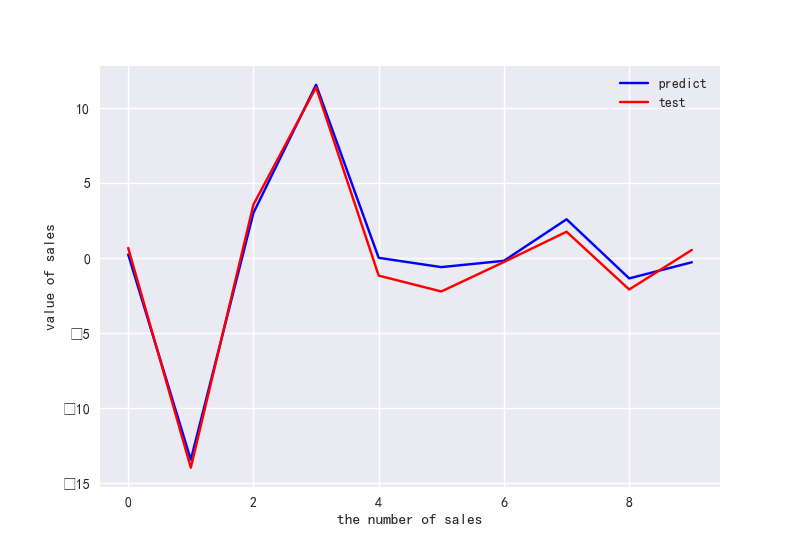

附錄：

相應的引數說明。 
fit_intercept: 布林型，預設為true 
說明：是否對訓練資料進行中心化。如果該變數為false，則表明輸入的資料已經進行了中心化，在下面的過程裡不進行中心化處理；否則，對輸入的訓練資料進行中心化處理 
normalize布林型，預設為false 
說明：是否對資料進行標準化處理 
copy_X 布林型，預設為true 
說明：是否對X複製，如果選擇false，則直接對原資料進行覆蓋。（即經過中心化，標準化後，是否把新資料覆蓋到原資料上） 
**n_jobs整型， 預設為1 
說明：計算時設定的任務個數(number of jobs)。如果選擇-1則代表使用所有的CPU。這一引數的對於目標個數>1（n_targets>1）且足夠大規模的問題有加速作用。 
返回值：

coef_ 陣列型變數， 形狀為(n_features,)或(n_targets, n_features) 
說明：對於線性迴歸問題計算得到的feature的係數。如果輸入的是多目標問題，則返回一個二維陣列(n_targets, n_features)；如果是單目標問題，返回一個一維陣列 (n_features,)。 
intercept_ 陣列型變數 
說明：線性模型中的獨立項。

注：該演算法僅僅是scipy.linalg.lstsq經過封裝後的估計器。

方法：

decision_function(X) 對訓練資料X進行預測 
fit(X, y[, n_jobs]) 對訓練集X, y進行訓練。是對scipy.linalg.lstsq的封裝 
get_params([deep]) 得到該估計器(estimator)的引數。 
predict(X) 使用訓練得到的估計器對輸入為X的集合進行預測（X可以是測試集，也可以是需要預測的資料）。 
score(X, y[,]sample_weight) 返回對於以X為samples，以y為target的預測效果評分。 
set_params(**params) 設定估計器的引數

decision_function(X) 和predict(X)都是利用預估器對訓練資料X進行預測，其中decision_function(X)包含了對輸入資料的型別檢查，以及當前物件是否存在coef_屬性的檢查，是一種“安全的”方法，而predict是對decision_function的呼叫。

score(X, y[,]sample_weight) 定義為(1-u/v)，其中u = （（y_true - y_pred）**2）.sum()，而v=((y_true-y_true.mean())**2).mean() 
最好的得分為1.0，一般的得分都比1.0低，得分越低代表結果越差。 
其中sample_weight為(samples_n,)形狀的向量，可以指定對於某些sample的權值，如果覺得某些資料比較重要，可以將其的權值設定的大一些。

例子：

from sklearn import linear_model
clf = linear_model.LinearRegression()
clf.fit ([[0, 0], [1, 1], [2, 2]], [0, 1, 2])
LinearRegression(copy_X=True, fit_intercept=True, n_jobs=1, normalize=False)
clf.coef_
array([ 0.5,  0.5])

相關知識點：

LOC函式：https://blog.csdn.net/weixin_39501270/article/details/76833836

Train_test_split函式：https://www.cnblogs.com/bonelee/p/8036024.html