Caffe 例項筆記 1 CaffeNet從訓練到分類及視覺化引數特徵微調

阿新 • • 發佈：2019-01-26

本文主要分四部分
1. 在命令列進行訓練
2. 使用pycaffe進行分類及特徵視覺化
3. 進行微調，將caffenet使用在圖片風格的預測上

1 使用caffeNet訓練自己的資料集

1.1 建立lmdb

使用對應的資料集建立lmdb：
這裡使用 examples/imagenet/create_imagenet.sh，需要更改其路徑和尺寸設定的選項，為了減小更改的數目，這裡並沒有自己新建立一個資料夾，而是直接使用了原來的imagenet的資料夾，而且將train.txt,val.txt都放置於/data/ilsvrc12中，

TRAIN_DATA_ROOT=/home/beatree/caffe-rc3/examples/imagenet/train/ 

VAL_DATA_ROOT=/home/beatree/caffe-rc3/examples/imagenet/val/

RESIZE=true

注意下面的地址的含義：

echo "Creating train lmdb..."

GLOG_logtostderr=1 $TOOLS/convert_imageset \
    --resize_height=$RESIZE_HEIGHT \
    --resize_width=$RESIZE_WIDTH \
    --shuffle \
    $TRAIN_DATA_ROOT \
    $DATA/train.txt \
    $EXAMPLE 
/ilsvrc12_train_lmdb

主要用了tools裡的convert_imageset

1.2 計算均值

模型需要我們從每張圖片減去均值,所以我們需要獲得訓練的均值，直接利用./examples/imagenet/make_imagenet_mean.sh建立均值檔案binaryproto，如果之前建立了新的路徑，這裡同樣需要修改sh檔案裡的路徑。
這裡的主要語句是

$TOOLS/compute_image_mean $EXAMPLE/ilsvrc12_train_lmdb \
  $DATA/imagenet_mean.binaryproto

如果顯示Check failed: size_in_datum == data_size () Incorrect data field size

說明上一步的圖片沒有統一尺寸

1.3 設定網路及求解器

這裡是利用原文的網路設定tain_val.prototxt和slover.prototext，在models/bvlc_reference_caffenet/solver.prototxt路徑中，這裡的訓練和驗證的網路基本一樣用 include { phase: TRAIN } or include { phase: TEST }和來區分，其兩點不同之處具體為：

transform_param {
    mirror: true#不同1：訓練集會randomly mirrors the input image
    crop_size: 227
    mean_file: "data/ilsvrc12/imagenet_mean.binaryproto"
  }
data_param {
    source: "examples/imagenet/ilsvrc12_train_lmdb"#不同2：來源不同
    batch_size: 32#原文很大，顯示卡比較弱的會記憶體不足，這裡改為了32，這裡根據需要更改，驗證集和訓練集的設定也不一樣
    backend: LMDB
  }

另外在輸出層也有不同，訓練時的loss需要用來進行反向傳遞，而val就不需要了。
solver.protxt的改動：
根據

net: "/home/beatree/caffe-rc3/examples/imagenet/train_val.prototxt"#網路配置存放地址
test_iter: 4， 每個批次是50，一共200個
test_interval: 300 #每300次測試一次
base_lr: 0.01 #是基礎學習率,因為資料量小,0.01 就會下降太快了,因此可以改成 0.001，這裡博主沒有改
lr_policy: "step" #lr可以變化
gamma: 0.1 #學習率變化的比率
stepsize: 300
display: 20 #20層顯示一次
max_iter: 1200 一共迭代1200次
momentum: 0.9
weight_decay: 0.0005
snapshot: 600 #每600存一個狀態
snapshot_prefix: "/home/beatree/caffe-rc3/examples/imagenet/"#狀態存放地址

1.4 訓練

使用上面的配置訓練，得到的結果準確率僅僅是0.2+，資料集的製作者迭代了12000次得到0.5的準確率

1.5 其他

1.5.1 檢視時間使用情況

./build/tools/caffe time --model=models/bvlc_reference_caffenet/train_val.prototxt

我的時間使用情況

Average Forward pass: 3490.86 ms.
Average Backward pass: 5666.73 ms.
Average Forward-Backward: 9157.66 ms.
Total Time: 457883 ms.

1.5.2 恢復資料

如果我們在訓練途中就停電或者有了其他的情況，我們可以通過之前儲存的狀態恢復資料，使用的時候直接新增–snapshot引數即可，如：

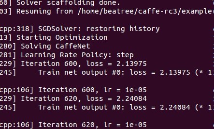
./build/tools/caffe train --solver=models/bvlc_reference_caffenet/solver.prototxt --snapshot=models/bvlc_reference_caffenet/caffenet_train_iter_10000.solverstate

這時候執行會從snapshot開始繼續執行，如從第600迭代時執行：
這裡寫圖片描述

1.5.3 c++ 提取特徵

when everything necessary is in place:

./build/tools/extract_features.bin models/bvlc_reference_caffenet/bvlc_reference_caffenet.caffemodel examples/_temp/imagenet_val.prototxt fc7 examples/_temp/features 10 leveldb

the features are stored to LevelDB examples/_temp/features.

1.5.4 使用c++分類

對於c++的學習應該讀讀tools/caffe.cpp裡的程式碼。
其分類命令如下：

 ./build/examples/cpp_classification/classification.bin \ models/bvlc_reference_caffenet/deploy.prototxt \ models/bvlc_reference_caffenet/bvlc_reference_caffenet.caffemodel \ data/ilsvrc12/imagenet_mean.binaryproto \ data/ilsvrc12/synset_words.txt \ examples/images/cat.jpg

2 使用pycaffe分類

2.1 import

首先載入環境：



# set up Python environment: numpy for numerical routines, and matplotlib for plotting
import numpy as np
import matplotlib.pyplot as plt
# display plots in this notebook
%matplotlib inline#這裡由於ipython啟動時移除了 pylab 啟動引數，所以需要使用這種格式檢視，官網介紹http://ipython.org/ipython-doc/stable/interactive/reference.html#plotting-with-matplotlib：
#To start IPython with matplotlib support, use the --matplotlib switch. If IPython is already running, you can run the %matplotlib magic. If no arguments are given, IPython will automatically detect your choice of matplotlib backend. You can also request a specific backend with %matplotlib backend, where backend must be one of: ‘tk’, ‘qt’, ‘wx’, ‘gtk’, ‘osx’. In the web notebook and Qt console, ‘inline’ is also a valid backend value, which produces static figures inlined inside the application window instead of matplotlib’s interactive figures that live in separate windows.

# set display defaults
#關於rcParams函式http://matplotlib.org/api/matplotlib_configuration_api.html#matplotlib.rcParams
plt.rcParams['figure.figsize'] = (10, 10)        # large images
plt.rcParams['image.interpolation'] = 'nearest'  # don't interpolate: show square pixels
plt.rcParams['image.cmap'] = 'gray'  # use grayscale output rather than a (potentially misleading) color heatmap

然後

import caffe#如果沒有設定好路徑可能發現不了caffe，需要import sys cafe_root='你的路徑'，sys.path.insert(0,caffe_root+'python')之後再import caffe

下面下載模型，由於上面剛開始我們用的資料不是imagenet，現在我們直接下載一個模型，可能你的python中沒有yaml，這裡可以用pip安裝（終端裡）：

sudo apt-get install python-pip
pip install pyyaml
cd #你的caffe root
./scripts/download_model_binary.py /home/beatree/caffe-rc3/model
/bvlc_reference_caffenet
#其他的網路路徑如下：models/bvlc_alexnet  models/bvlc_reference_rcnn_ilsvrc13  models/bvlc_googlenet  model zoo的連線http://caffe.berkeleyvision.org/model_zoo.html，模型一共232m

2.2 模型載入

caffe.set_mode_cpu()#使用cpu模式
model_def='/home/beatree/caffe-rc3/models/bvlc_reference_caffenet/deploy.prototxt'
model_weights='/home/beatree/caffe-rc3/models/bvlc_reference_caffenet/bvlc_reference_caffenet.caffemodel'
net=caffe.Net(model_def,
              model_weights,
              caffe.TEST)

mu=np.load('/home/beatree/caffe-rc3/python/caffe/imagenet/ilsvrc_2012_mean.npy')
mu=mu.mean(1).mean(1)

mu長成下面這個樣子：

array([[[ 110.17708588,  110.45915222,  110.68373108, ...,  110.9342804 ,
          110.79355621,  110.5134201 ],
        [ 110.42878723,  110.98564148,  111.27901459, ...,  111.55055237,
          111.30683136,  110.6951828 ],
        [ 110.525177  ,  111.19493103,  111.54753113, ...,  111.81067657,
          111.47111511,  110.76550293],
          ……

得到bgr的均值

print 'mean-subtracted values:', zip('BGR', mu)

mean-subtracted values: [('B', 104.0069879317889), ('G', 116.66876761696767), ('R', 122.6789143406786)]

matplotlib載入的image是畫素[0-1],圖片的資料格式[weight,high,channels]，RGB 而caffe載入的圖片需要的是[0-255]畫素，資料格式[channels,weight,high],BGR，那麼就需要轉換，這裡用了 caffe.io.Transformer,可以使用help()來獲得相關資訊，他的功能有
preprocess(self, in_, data)
set_channel_swap(self, in_, order)
set_input_scale(self, in_, scale)
set_mean(self, in_, mean)
set_raw_scale(self, in_, scale)
set_transpose(self, in_, order)

# create transformer for the input called 'data'
transformer = caffe.io.Transformer({'data': net.blobs['data'].data.shape})#net.blobs['data'].data.shape=(10, 3, 227, 227)

transformer.set_transpose('data', (2,0,1))  # move image channels to outermost dimension第一個變成了channels
transformer.set_mean('data', mu)            # subtract the dataset-mean value in each channel
transformer.set_raw_scale('data', 255)      # rescale from [0, 1] to [0, 255]
transformer.set_channel_swap('data', (2,1,0))  # swap channels from RGB to BGR

2.3 cpu 分類

這裡可以準備開始分類了，下面改變輸入size的步驟也可以跳過，這裡batchsize設定為50只是為了演示用，實際我們只對一張圖片進行分類。

# set the size of the input (we can skip this if we're happy
#  with the default; we can also change it later, e.g., for different batch sizes)
net.blobs['data'].reshape(50,        # batch size
                          3,         # 3-channel (BGR) images
                          227, 227)  # image size is 227x227

image = caffe.io.load_image( 'path/to/images/cat.jpg')
transformed_image = transformer.preprocess('data', image)
plt.imshow(image)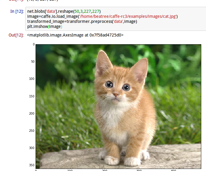

這裡寫圖片描述
得到一個可愛的小貓,接下來看一看模型是不是認為她是不是小貓

# copy the image data into the memory allocated for the net
net.blobs['data'].data[...] = transformed_image

### perform classification
output = net.forward()

output_prob = output['prob'][0]  # the output probability vector for the first image in the batch

print 'predicted class is:', output_prob.argmax(),output_prob[output_prob.argmax()]

得到結果：

predicted calss is 281 0.312436

也就是第281種最有可能，概率比重是0.312436
那麼第231種是不是貓呢，讓我們接著看

# load ImageNet labels
labels_file = caffe_root + 'data/ilsvrc12/synset_words.txt'#如果沒有這個檔案，須執行/data/ilsvrc12/get_ilsvrc_aux.sh
labels = np.loadtxt(labels_file, str, delimiter='\t')

print 'output label:', labels[output_prob.argmax()]

結果是answer is n02123045 tabby, tabby cat連花紋都判斷對了。接下來讓我們進一步觀察判斷的結果：

# sort top five predictions from softmax output
top_inds = output_prob.argsort()[::-1][:5]  # reverse sort and take five largest items

print 'probabilities and labels:'
zip(output_prob[top_inds], labels[top_inds])

得到的結果是：

[(0.31243584, 'n02123045 tabby, tabby cat'),#虎斑貓
 (0.2379715, 'n02123159 tiger cat'),#虎貓
 (0.12387265, 'n02124075 Egyptian cat'),#埃及貓
 (0.10075713, 'n02119022 red fox, Vulpes vulpes'),#赤狐
 (0.070957303, 'n02127052 lynx, catamount')]#猞猁，山貓

2.4 對比GPU

現在對比下GPU與CPU的效能表現
首先看看cpu每次（50 batch size）向前執行的時間：

%timeit net.forward（）

%timeit能自動選擇執行的次數求平均執行時間，這裡我的執行時間是1 loops, best of 3: 5.29 s per loop，官網的是1.42,差距
接下來看GPU的執行時間：

caffe.set_device(0)
caffe.set_mode_gpu()
net.forward()
%timeit net.forward()

1 loops, best of 3: 507 ms per loop（官網是70.2ms）,慢了好多的說

2.5 檢視中間輸出

首先我們看下網路的結構及每層輸出的shape，其形式應該是（batchsize，channeldim，height，weight）

# for each layer, show the output shape
for layer_name, blob in net.blobs.iteritems():
    print layer_name + '\t' + str(blob.data.shape)

得到的結果如下：

data    (50, 3, 227, 227)
conv1   (50, 96, 55, 55)
pool1   (50, 96, 27, 27)
norm1   (50, 96, 27, 27)
conv2   (50, 256, 27, 27)
pool2   (50, 256, 13, 13)
norm2   (50, 256, 13, 13)
conv3   (50, 384, 13, 13)
conv4   (50, 384, 13, 13)
conv5   (50, 256, 13, 13)
pool5   (50, 256, 6, 6)
fc6 (50, 4096)
fc7 (50, 4096)
fc8 (50, 1000)
prob    (50, 1000)

現在看其引數的樣子，函式為net.params,其中weight的樣子應該是（output_channels,input_channels,filter_height,flier_width）, biases的形狀只有一維（output_channels,）

for layer_name,parame in net.params.iteritems():
print layer_name+'\t'+str(param[0].shape),str(param[1].data.shape)#可以看出param裡0為weight1為biase

得到：

conv1   (96, 3, 11, 11) (96,)#輸入3通道，輸出96通道
conv2   (256, 48, 5, 5) (256,)#為什麼變成48了？看下方解釋
conv3   (384, 256, 3, 3) (384,)#這裡的輸入沒變
conv4   (384, 192, 3, 3) (384,)
conv5   (256, 192, 3, 3) (256,)
fc6 (4096, 9216) (4096,)#9216=25*3*3
fc7 (4096, 4096) (4096,)
fc8 (1000, 4096) (1000,)

可以看出只有卷基層和全連線層有引數
既然後了各個引數我們就初步解讀下caffenet：
首先第一層conv1其輸出結果的變化
這裡寫圖片描述，
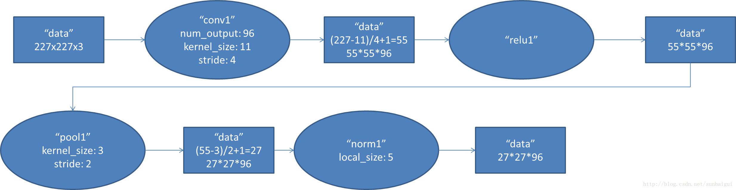
（圖片來自部落格http://blog.csdn.net/sunbaigui/article/details/39938097）
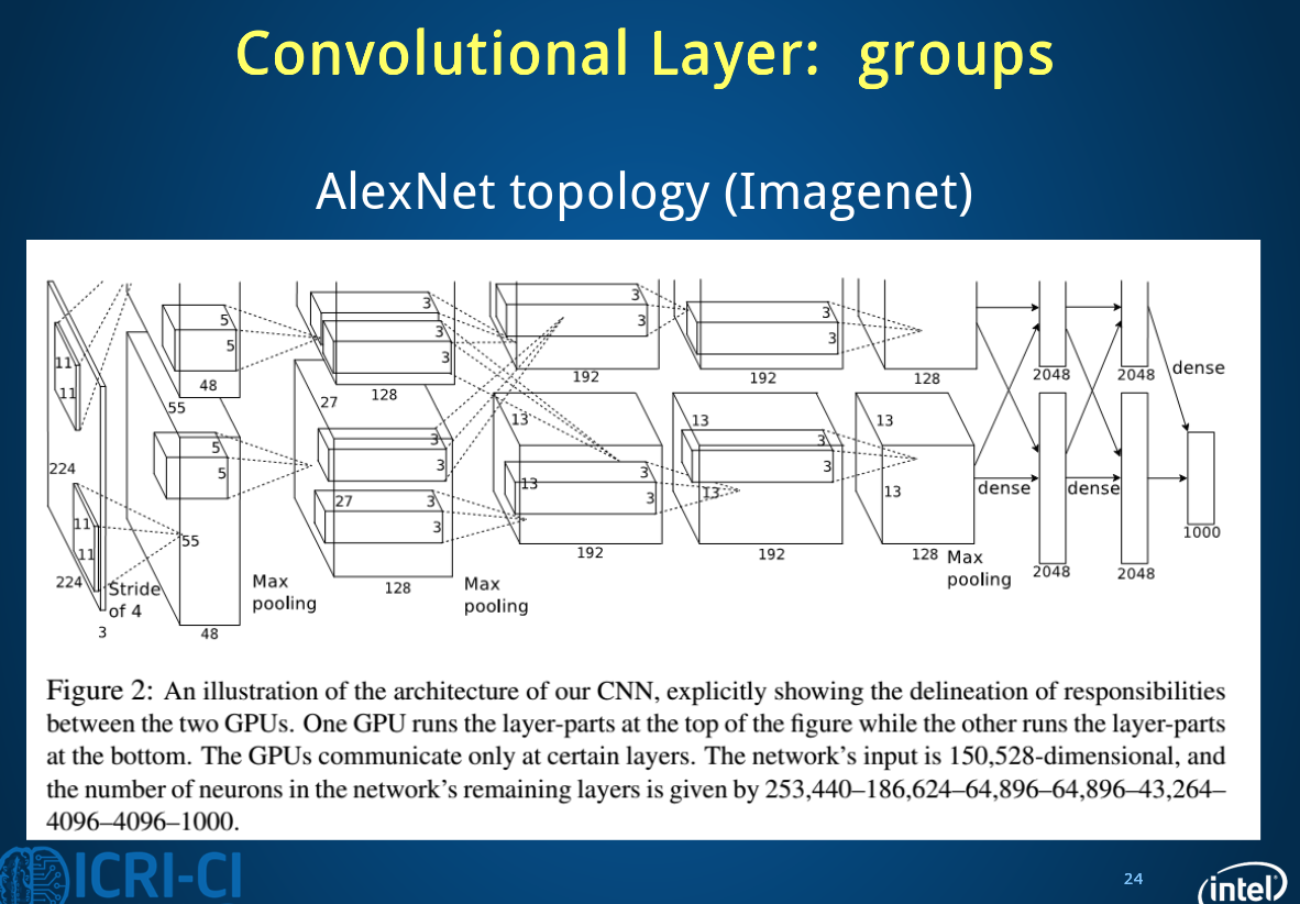
這一步應該可以理解，其權重的形式為(96, 3, 11, 11)
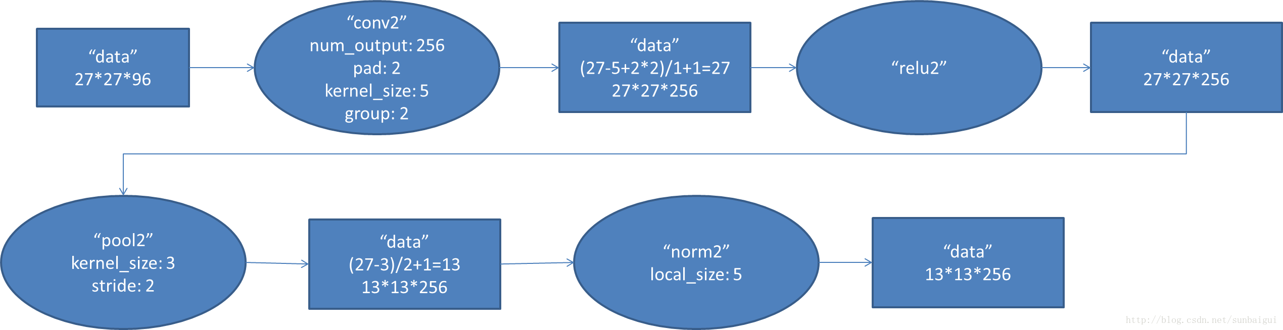
但是第二層的卷積層為什麼為(256, 48, 5, 5)，因為這裡多了一個group選項，在cs231n裡沒有提及，這裡的group=2，把輸入輸出分為了兩個組也就是輸入變成了96/2=48，
這裡寫圖片描述
全連線層fc6的資料流圖：

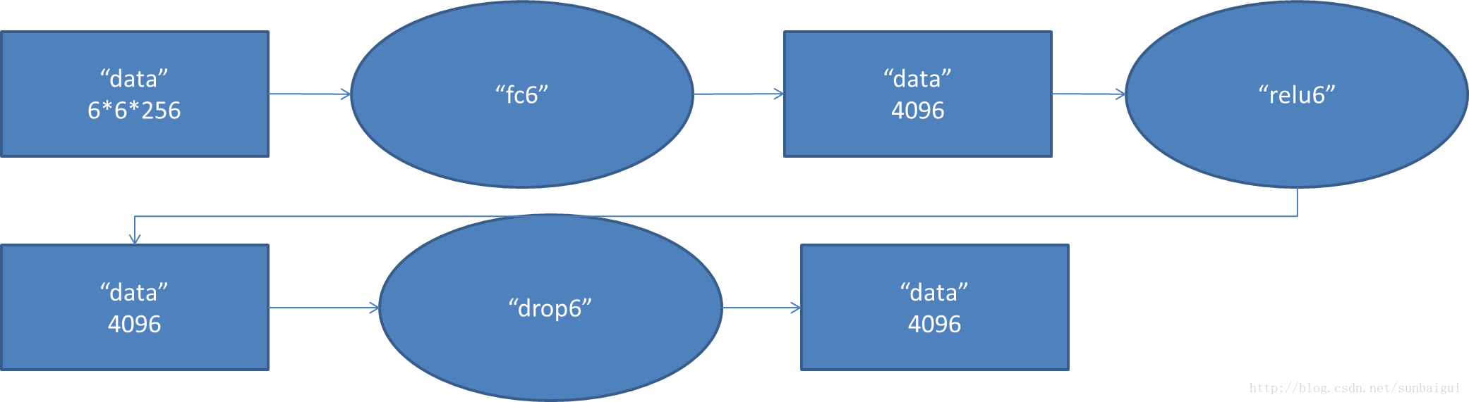
這是一張特拉維夫大學的ppt

下面進行視覺化操作，首先要定義一個函式方便以後呼叫，視覺化各層引數和結果:

def vis_square(data):
    """Take an array of shape (n, height, width) or (n, height, width, 3)
       and visualize each (height, width) thing in a grid of size approx. sqrt(n) by sqrt(n)"""
       #輸入為格式為數量，高，寬，（3），最終展示是在一個方形上

    # normalize data for display
    #首先將資料規則化
    data = (data - data.min()) / (data.max() - data.min())
    # force the number of filters to be square
    n = int(np.ceil(np.sqrt(data.shape[0])))
    #pad是補充的函式，paddign是每個緯度擴充的數量
    padding = (((0, n ** 2 - data.shape[0]),
               (0, 1), (0, 1))                 # add some space between filters，間隔的大小
               + ((0, 0),) * (data.ndim - 3))  # don't pad the last dimension (if there is one)如果有3通道，要保持其不變
    data = np.pad(data, padding, mode='constant', constant_values=0)  # pad with zero (black)這裡該為了黑色，可以更容易看出最後一列中拓展的樣子

    # tile the filters into an image
    data = data.reshape((n, n) + data.shape[1:]).transpose((0, 2, 1, 3) + tuple(range(4, data.ndim + 1)))
    data = data.reshape((n * data.shape[1], n * data.shape[3]) + data.shape[4:])
    plt.imshow(data)
    plt.axis('off')

以conv1為例，探究如果reshape的

filters = net.params['conv1'][0].data
vis_square(filters.transpose(0, 2, 3, 1))

得到的結果
這裡寫圖片描述
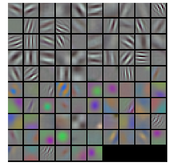
這裡conv1的權重，原來的shape是(96, 3, 11, 11)，其中輸出為96層，每個filter的大小是11 11 3（注意後面的3噢），每個filter經過滑動視窗（卷積）得到一張output，一共得到96個。（下圖是錯誤的，請去官網看正確的）
這裡寫圖片描述
首先進入vissquare之前要transpose–》（96，11，11，3）
輸入vis_square得到的padding是（0，4），（0，1），（0，1），（0，0）也就是經過padding之後變為（100，12，12，3），這時的12多出了一個邊框，第一個reshape(10,10,12,12,3),相當於原來100個圖片一排變為矩陣式排列，然後又經過transpose（0，2，1，3，4）—>（10，12，10，12，3）又經過第二個reshape（120，120，3）
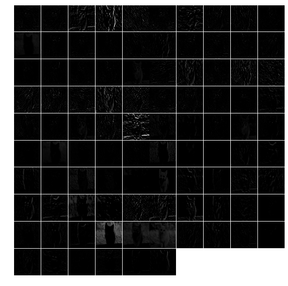
下面展示第一層filter輸出的特徵：

feat = net.blobs['conv1'].data[0, :36]#原輸出為（50，96，55，55），這裡取第一幅圖前36張
vis_square(feat)

？

如果取全部的96張會出現下面的情況：中間的分割線沒有了，為什麼呢？
這裡寫圖片描述
用上面的方法也可以檢視其他幾層的輸出。
對於全連線層的輸出需要用直方圖的形式：

feat = net.blobs['fc6'].data[0]
plt.subplot(2, 1, 1)
plt.plot(feat.flat)
plt.subplot(2, 1, 2)
_ = plt.hist(feat.flat[feat.flat > 0], bins=100)#bin統計某一個數段之間的數量

輸出分類結果：

feat = net.blobs['prob'].data[0]
plt.figure(figsize=(15, 3))
plt.plot(feat.flat)

大體就是這樣了，我們可以用自己的圖片來分類看看結果

2.6 總結

主要分類過程程式碼主要步驟：
1. 載入工具包
2. 設定顯示設定
3. 設定求解其set_mode_cup()/gpu()
4. 載入模型 net=caffe.Net(,,caffe.TEST)
5. transformer（包括載入均值）
6. 設定分類輸入size（batch size等）
7. 載入圖片並轉換（io.load_image(‘path’), transformer.preprocesss）
8. net.blobs[‘data’],data[…]=transformed_image
9. 向前計算output=net.forward
10. output_prob=output[‘prob’][0]
11. 載入synset_words.txt(np.loadtxt(,,))
12. 分類結果輸出 output_prob.argsort()[::-1][] ⋆⋆⋆⋆⋆
13. 展示各層輸出net.blobs.iteritems()
14. 展示各層引數net.params.iteritems()
15. 視覺化注意pad和reshape，transpose的運用
16. net.params[‘name’][0].data
17. net.blobs[‘name’].data[0,:36]
18. net.blobs[‘prob’].data[0]#每個圖片都有不同的輸出所以後面加了個【0】

3 Fine-tuning

Now we will fine-tune the model we trained above on a different dataset to predict image style. we have 80000 images to train on. There will some changes :
1. we will change the name of the last layer form fc8 to fc8_flickr in our prototxt, it will begin training with random weights.
2. decrease base_lr andboost the lr_mult on the newly introduced layer.
3. set stepsize to a lower value. So the learning rate to go down faster
4. So in the solver.prototxt,we can find the base_lr is 0.001 from 0.01,and the stepsize is become to 20000 from 100000.

3.1 cmdcaffe

3.1.1 download dataset & model

we will only download 2000 images

python ./examples/finetune_flickr_style/assemble_data.py --workers=-1 --images=2000 --seed 831486

we have already download the model in the previous step

3.1.2 fine tune

let’s see some information in the new train_val.prototxt:
1. ImageData later

layer{
name:"data"
type:"ImageData"
...
transform_param{#預處理
  mirror=true
  crop_size:227#切割
  mean_file:"yourpath.binaryproto"}
 image_data_param{
   source:"" 
   batch_size: 
   new_height: 
   new_width: }}

另外加了一層規則化的dropout層。
在fc8_flickr層的lr_mult分別為10和20

./build/tools/caffe train -solver models/finetune_flick_style/solver.prototxt -weithts
models/bvlc_reference_caffenet/bvlc_reference_caffenet.caffemodel -gpu 0

3.2 pycaffe

some functions in python ：

import tempfile
image=np.around()
image=np.require(image,dtype=np.uint8)
assert os.path.exists(weights)#宣告，如果路徑不存在會報錯
。。。

在這一部分，通過ipython notebook定義了完整的網路與solver，並比較了微調模型與直接訓練模型的差異，程式碼相對來說更加具體，由於下一邊部落格相關敘述比較仔細，這裡就不重複了，但是還是很有必要按照官網來一遍的。

3.3 主要步驟

3.3.1 下載caffenet模型，下載Flickr資料

weights=’…..caffemodel’

3.3.2 defining and runing the nets

def caffenet():
   n=caffe.NetSpec()
   n.data=data 
   n.conv1,n.relu1= 
   ...  
   if train: 
      n.drop6=fc7input=L.Dropout(n.relu6,in_place=True) 
   else:  
      fc7input=n.relu6   
   if...else...   
   fc8=L.InnerProduct(fc8input,num_output=num_clsasses,param=learned_param) 
   n.__setattr__(classifier_name,fc8)#classifier_name='fc8_flickr'  
   if not train: 
       n.probs=L.Softmax(fc8)  
    if label is not None: 
       n.label=label 
       n.loss=L.SoftmaxWithLoss(fc8,n.label)
       n.acc=L.Accuracy(fc8,n.label) 
    with tempfile.NamedTemporaryFile(delete=False)as f: 
    f.write(str(n.to_proto())) 
    return f.name

3.3.3 dummy data imagenet

L.DummyData(shape=dict(dim=[1,3,227,227])) 
imagenet_net_filename=caffenet(data,train=False) 
imagenet_net=caffe.Net(imagenet_net_filename,weights,caffe.TEST)

3.3.4 style_net

have the same architecture as CaffeNet,but with differences in the input and output：

def style_net(traih=True,Learn_all=False,subset=None):
   if subset is None:
      subset ='train' if train else 'test' 
   source='path/%s.txt'%subset 
   trainsfor_param=dict(mirror=train,crop_size=227,meanfile='path/xx.binaryproto') 
   style_data,style_label=L.ImageData(transform_param=,source=,batch_size=,new_height=,new_width=,ntop=2) 
   return caffenet(data=style_data,label=style_label,train=train,num_classes=20,classifier_name='fc8_filcker',learn_all=learn_all)

3.3.5 對比untrained_style_net,imagenet_net

3.3.6 training the style classifier

from caffe.proto import caffe_pb2 
def solver(): 
s=caffe_pb2.SloverParameter() 
s.train_net=train_net_path 
if test_net_path is not None: 
   ...  
 s.xx=xxx 
with temfile.Nxx as f: 
    f.write(str(s)) 
    return f.name

bulit/tools/caffe train \ -solver models/path/sovler.prototxt\ -weights /path/.caffemodel\ gpu 0

def run_solvers():
   for it in range(niter):
      for name, s in solvers:   
         s.step(1) 
         loss[][],acc[][]=(s.net.blobs[b].data.copy()for b in blobs) 
         if it % disp_interval==0 or it+1 
            ...print ...    
         weight_dir=tempfile.mkdtemp() 
         weights={}  
         for name,s in solvers:    
             filename=   
             weights[name]=os.path.join(weight_dir,filename)  
             s.net.save(weights[name])      
          return loss,acc,weights

3.3.7 對比預訓練效果

預訓練多了一步：style_solver.net.copy_from(weights)

3.3.8 end-to-end finetuning for style

learn_all=Ture

Caffe 例項筆記 1 CaffeNet從訓練到分類及視覺化引數特徵 微調