人臉識別

Face Recognition for the Happy House

from keras.models import Sequential
from keras.layers import Conv2D, ZeroPadding2D, Activation, Input, concatenate
from keras.models import Model
from keras.layers.normalization import BatchNormalization
from keras.layers.pooling import MaxPooling2D, AveragePooling2D
from
 
 keras.layers.merge import Concatenate
from keras.layers.core import Lambda, Flatten, Dense
from keras.initializers import glorot_uniform
from keras.engine.topology import Layer
from keras import backend as K
K.set_image_data_format('channels_first')
import cv2
import os
import numpy as np
from numpy import
 
 genfromtxt
import pandas as pd
import tensorflow as tf
from fr_utils import *
from inception_blocks_v2 import *

%matplotlib inline
%load_ext autoreload
%autoreload 2

np.set_printoptions(threshold=np.nan)

0 - Naive Face Verification

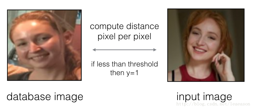
In Face Verification, you’re given two images and you have to tell if they are of the same person. The simplest way to do this is to compare the two images pixel-by-pixel. If the distance between the raw images are less than a chosen threshold, it may be the same person!

1 - Encoding face images into a 128-dimensional vector

1.1 - Using an ConvNet to compute encodings

The FaceNet model takes a lot of data and a long time to train. So following common practice in applied deep learning settings, let’s just load weights that someone else has already trained. The network architecture follows the Inception model from Szegedy et al.. We have provided an inception network implementation. You can look in the file inception_blocks.py to see how it is implemented (do so by going to “File->Open…” at the top of the Jupyter notebook).

FRmodel = faceRecoModel(input_shape=(3, 96, 96))
print("Total Params:", FRmodel.count_params())

Total Params: 3743280
By using a 128-neuron fully connected layer as its last layer, the model ensures that the output is an encoding vector of size 128. You then use the encodings the compare two face images as follows:

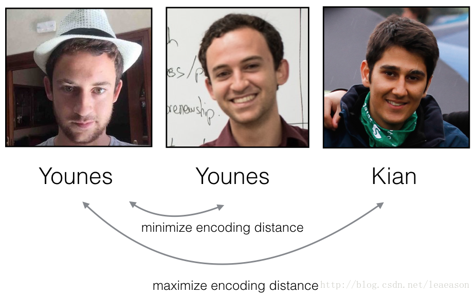
So, an encoding is a good one if:
The encodings of two images of the same person are quite similar to each other
The encodings of two images of different persons are very different
The triplet loss function formalizes this, and tries to “push” the encodings of two images of the same person (Anchor and Positive) closer together, while “pulling” the encodings of two images of different persons (Anchor, Negative) further apart.

1.2 - The Triplet Loss

# GRADED FUNCTION: triplet_loss

def triplet_loss(y_true, y_pred, alpha = 0.2):
    """
    Implementation of the triplet loss as defined by formula (3)

    Arguments:
    y_true -- true labels, required when you define a loss in Keras, you don't need it in this function.
    y_pred -- python list containing three objects:
            anchor -- the encodings for the anchor images, of shape (None, 128)
            positive -- the encodings for the positive images, of shape (None, 128)
            negative -- the encodings for the negative images, of shape (None, 128)

    Returns:
    loss -- real number, value of the loss
    """

    anchor, positive, negative = y_pred[0], y_pred[1], y_pred[2]

    ### START CODE HERE ### (≈ 4 lines)
    # Step 1: Compute the (encoding) distance between the anchor and the positive
    pos_dist = tf.reduce_sum(tf.square(tf.subtract(y_pred[0],y_pred[1])))
    # Step 2: Compute the (encoding) distance between the anchor and the negative
    neg_dist = tf.reduce_sum(tf.square(tf.subtract(y_pred[0],y_pred[2])))
    # Step 3: subtract the two previous distances and add alpha.
    basic_loss = tf.add(tf.subtract(pos_dist,neg_dist),alpha)
    # Step 4: Take the maximum of basic_loss and 0.0. Sum over the training examples.
    loss = tf.reduce_sum(tf.maximum(basic_loss,0.0))
    ### END CODE HERE ###

    return loss

with tf.Session() as test:
    tf.set_random_seed(1)
    y_true = (None, None, None)
    y_pred = (tf.random_normal([3, 128], mean=6, stddev=0.1, seed = 1),
              tf.random_normal([3, 128], mean=1, stddev=1, seed = 1),
              tf.random_normal([3, 128], mean=3, stddev=4, seed = 1))
    loss = triplet_loss(y_true, y_pred)

    print("loss = " + str(loss.eval()))

loss = 350.026

2 - Loading the trained model

FRmodel.compile(optimizer = 'adam', loss = triplet_loss, metrics = ['accuracy'])
load_weights_from_FaceNet(FRmodel)

3 - Applying the model

Back to the Happy House! Residents are living blissfully since you implemented happiness recognition for the house in an earlier assignment.
However, several issues keep coming up: The Happy House became so happy that every happy person in the neighborhood is coming to hang out in your living room. It is getting really crowded, which is having a negative impact on the residents of the house. All these random happy people are also eating all your food.
So, you decide to change the door entry policy, and not just let random happy people enter anymore, even if they are happy! Instead, you’d like to build a Face verification system so as to only let people from a specified list come in. To get admitted, each person has to swipe an ID card (identification card) to identify themselves at the door. The face recognition system then checks that they are who they claim to be.

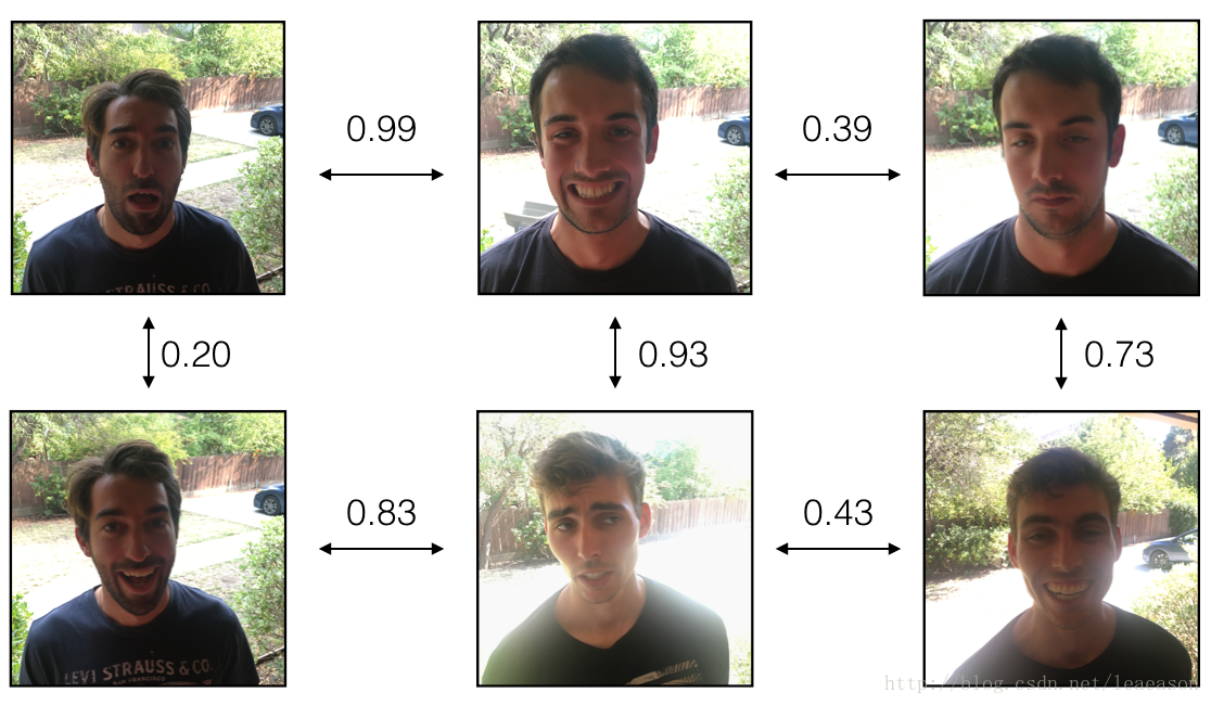
3.1 - Face Verification

database = {}
database["danielle"] = img_to_encoding("images/danielle.png", FRmodel)
database["younes"] = img_to_encoding("images/younes.jpg", FRmodel)
database["tian"] = img_to_encoding("images/tian.jpg", FRmodel)
database["andrew"] = img_to_encoding("images/andrew.jpg", FRmodel)
database["kian"] = img_to_encoding("images/kian.jpg", FRmodel)
database["dan"] = img_to_encoding("images/dan.jpg", FRmodel)
database["sebastiano"] = img_to_encoding("images/sebastiano.jpg", FRmodel)
database["bertrand"] = img_to_encoding("images/bertrand.jpg", FRmodel)
database["kevin"] = img_to_encoding("images/kevin.jpg", FRmodel)
database["felix"] = img_to_encoding("images/felix.jpg", FRmodel)
database["benoit"] = img_to_encoding("images/benoit.jpg", FRmodel)
database["arnaud"] = img_to_encoding("images/arnaud.jpg", FRmodel)

# GRADED FUNCTION: verify

def verify(image_path, identity, database, model):
    """
    Function that verifies if the person on the "image_path" image is "identity".

    Arguments:
    image_path -- path to an image
    identity -- string, name of the person you'd like to verify the identity. Has to be a resident of the Happy house.
    database -- python dictionary mapping names of allowed people's names (strings) to their encodings (vectors).
    model -- your Inception model instance in Keras

    Returns:
    dist -- distance between the image_path and the image of "identity" in the database.
    door_open -- True, if the door should open. False otherwise.
    """

    ### START CODE HERE ###

    # Step 1: Compute the encoding for the image. Use img_to_encoding() see example above. (≈ 1 line)
    encoding = img_to_encoding(image_path,model)

    # Step 2: Compute distance with identity's image (≈ 1 line)
    dist = np.linalg.norm(encoding-database[identity])

    # Step 3: Open the door if dist < 0.7, else don't open (≈ 3 lines)
    if dist<0.7:
        print("It's " + str(identity) + ", welcome home!")
        door_open = True
    else:
        print("It's not " + str(identity) + ", please go away")
        door_open = False

    ### END CODE HERE ###

    return dist, door_open

verify("images/camera_0.jpg", "younes", database, FRmodel)

3.2 - Face Recognition

Your face verification system is mostly working well. But since Kian got his ID card stolen, when he came back to the house that evening he couldn’t get in!
To reduce such shenanigans, you’d like to change your face verification system to a face recognition system. This way, no one has to carry an ID card anymore. An authorized person can just walk up to the house, and the front door will unlock for them!
You’ll implement a face recognition system that takes as input an image, and figures out if it is one of the authorized persons (and if so, who). Unlike the previous face verification system, we will no longer get a person’s name as another input.
Exercise: Implement who_is_it(). You will have to go through the following steps:
Compute the target encoding of the image from image_path
Find the encoding from the database that has smallest distance with the target encoding.
Initialize the min_dist variable to a large enough number (100). It will help you keep track of what is the closest encoding to the input’s encoding.
Loop over the database dictionary’s names and encodings. To loop use for (name, db_enc) in database.items().
Compute L2 distance between the target “encoding” and the current “encoding” from the database.
If this distance is less than the min_dist, then set min_dist to dist, and identity to name.

# GRADED FUNCTION: who_is_it

def who_is_it(image_path, database, model):
    """
    Implements face recognition for the happy house by finding who is the person on the image_path image.

    Arguments:
    image_path -- path to an image
    database -- database containing image encodings along with the name of the person on the image
    model -- your Inception model instance in Keras

    Returns:
    min_dist -- the minimum distance between image_path encoding and the encodings from the database
    identity -- string, the name prediction for the person on image_path
    """

    ### START CODE HERE ### 

    ## Step 1: Compute the target "encoding" for the image. Use img_to_encoding() see example above. ## (≈ 1 line)
    encoding = img_to_encoding(image_path,model)

    ## Step 2: Find the closest encoding ##

    # Initialize "min_dist" to a large value, say 100 (≈1 line)
    min_dist = 100

    # Loop over the database dictionary's names and encodings.
    for (name, db_enc) in database.items():

        # Compute L2 distance between the target "encoding" and the current "emb" from the database. (≈ 1 line)
        dist = np.linalg.norm(encoding-db_enc)

        # If this distance is less than the min_dist, then set min_dist to dist, and identity to name. (≈ 3 lines)
        if dist<min_dist:
            min_dist = dist
            identity = name

    ### END CODE HERE ###

    if min_dist > 0.7:
        print("Not in the database.")
    else:
        print ("it's " + str(identity) + ", the distance is " + str(min_dist))

    return min_dist, identity

who_is_it("images/camera_0.jpg", database, FRmodel)

Deep Learning & Art: Neural Style Transfer

Welcome to the second assignment of this week. In this assignment, you will learn about Neural Style Transfer. This algorithm was created by Gatys et al. (2015) (https://arxiv.org/abs/1508.06576).
In this assignment, you will:
Implement the neural style transfer algorithm
Generate novel artistic images using your algorithm
Most of the algorithms you’ve studied optimize a cost function to get a set of parameter values. In Neural Style Transfer, you’ll optimize a cost function to get pixel values!

import os
import sys
import scipy.io
import scipy.misc
import matplotlib.pyplot as plt
from matplotlib.pyplot import imshow
from PIL import Image
from nst_utils import *
import numpy as np
import tensorflow as tf

%matplotlib inline

1 - Problem Statement

Neural Style Transfer (NST) is one of the most fun techniques in deep learning. As seen below, it merges two images, namely, a “content” image (C) and a “style” image (S), to create a “generated” image (G). The generated image G combines the “content” of the image C with the “style” of image S.
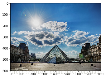
In this example, you are going to generate an image of the Louvre museum in Paris (content image C), mixed with a painting by Claude Monet, a leader of the impressionist movement (style image S).

2 - Transfer Learning

Neural Style Transfer (NST) uses a previously trained convolutional network, and builds on top of that. The idea of using a network trained on a different task and applying it to a new task is called transfer learning.
Following the original NST paper (https://arxiv.org/abs/1508.06576), we will use the VGG network. Specifically, we’ll use VGG-19, a 19-layer version of the VGG network. This model has already been trained on the very large ImageNet database, and thus has learned to recognize a variety of low level features (at the earlier layers) and high level features (at the deeper layers).
Run the following code to load parameters from the VGG model. This may take a few seconds.

3 - Neural Style Transfer

3.1 - Computing the content cost

content_image = scipy.misc.imread("images/louvre.jpg")
imshow(content_image)

# GRADED FUNCTION: compute_content_cost

def compute_content_cost(a_C, a_G):
    """
    Computes the content cost

    Arguments:
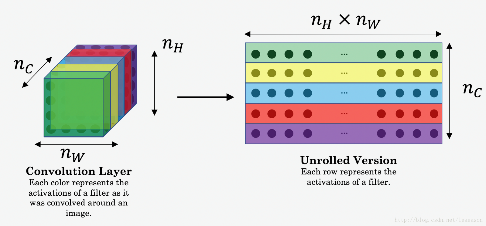
    a_C -- tensor of dimension (1, n_H, n_W, n_C), hidden layer activations representing content of the image C 
    a_G -- tensor of dimension (1, n_H, n_W, n_C), hidden layer activations representing content of the image G

    Returns: 
    J_content -- scalar that you compute using equation 1 above.
    """

    ### START CODE HERE ###
    # Retrieve dimensions from a_G (≈1 line)
    m, n_H, n_W, n_C = a_G.get_shape().as_list()

    # Reshape a_C and a_G (≈2 lines)
    a_C_unrolled = tf.reshape(a_C,shape=(n_H* n_W,n_C))
    a_G_unrolled = tf.reshape(a_G,shape=(n_H* n_W,n_C))

    # compute the cost with tensorflow (≈1 line)
    J_content = tf.reduce_sum(tf.square(tf.subtract(a_C_unrolled,a_G_unrolled)))/(4*n_H*n_W*n_C)
    ### END CODE HERE ###

    return J_content

tf.reset_default_graph()

with tf.Session() as test:
    tf.set_random_seed(1)
    a_C = tf.random_normal([1, 4, 4, 3], mean=1, stddev=4)
    a_G = tf.random_normal([1, 4, 4, 3], mean=1, stddev=4)
    J_content = compute_content_cost(a_C, a_G)
    print("J_content = " + str(J_content.eval()))

J_content = 6.76559

3.2 - Computing the style cost

3.2.1 - Style matrix

# GRADED FUNCTION: gram_matrix

def gram_matrix(A):
    """
    Argument:
    A -- matrix of shape (n_C, n_H*n_W)

    Returns:
    GA -- Gram matrix of A, of shape (n_C, n_C)
    """

    ### START CODE HERE ### (≈1 line)
    GA = tf.matmul(A,tf.transpose(A))
    ### END CODE HERE ###

    return GA

tf.reset_default_graph()

with tf.Session() as test:
    tf.set_random_seed(1)
    A = tf.random_normal([3, 2*1], mean=1, stddev=4)
    GA = gram_matrix(A)

    print("GA = " + str(GA.eval()))

GA = [[ 6.42230511 -4.42912197 -2.09668207]
[ -4.42912197 19.46583748 19.56387138]
[ -2.09668207 19.56387138 20.6864624 ]]

3.2.2 - Style cost

# GRADED FUNCTION: compute_layer_style_cost

def compute_layer_style_cost(a_S, a_G):
    """
    Arguments:
    a_S -- tensor of dimension (1, n_H, n_W, n_C), hidden layer activations representing style of the image S 
    a_G -- tensor of dimension (1, n_H, n_W, n_C), hidden layer activations representing style of the image G

    Returns: 
    J_style_layer -- tensor representing a scalar value, style cost defined above by equation (2)
    """

    ### START CODE HERE ###
    # Retrieve dimensions from a_G (≈1 line)
    m, n_H, n_W, n_C =  a_G.get_shape().as_list()

    # Reshape the images to have them of shape (n_C, n_H*n_W) (≈2 lines)
    a_S = tf.reshape(a_S,shape=(n_H*n_W,n_C))
    a_G = tf.reshape(a_G,shape=(n_H*n_W,n_C))

    # Computing gram_matrices for both images S and G (≈2 lines)
    GS = gram_matrix(tf.transpose(a_S))
    GG = gram_matrix(tf.transpose(a_G))

    # Computing the loss (≈1 line)
    J_style_layer = tf.reduce_sum(tf.square(tf.subtract(GS,GG)))/(4*(n_C*n_C)*(n_W * n_H) * (n_W * n_H))

    ### END CODE HERE ###

    return J_style_layer

tf.reset_default_graph()

with tf.Session() as test:
    tf.set_random_seed(1)
    a_S = tf.random_normal([1, 4, 4, 3], mean=1, stddev=4)
    a_G = tf.random_normal([1, 4, 4, 3], mean=1, stddev=4)
    J_style_layer = compute_layer_style_cost(a_S, a_G)

    print("J_style_layer = " + str(J_style_layer.eval()))

J_style_layer = 9.19028

3.2.3 Style Weights

def compute_style_cost(model, STYLE_LAYERS):
    """
    Computes the overall style cost from several chosen layers

    Arguments:
    model -- our tensorflow model
    STYLE_LAYERS -- A python list containing:
                        - the names of the layers we would like to extract style from
                        - a coefficient for each of them

    Returns: 
    J_style -- tensor representing a scalar value, style cost defined above by equation (2)
    """

    # initialize the overall style cost
    J_style = 0

    for layer_name, coeff in STYLE_LAYERS:

        # Select the output tensor of the currently selected layer
        out = model[layer_name]

        # Set a_S to be the hidden layer activation from the layer we have selected, by running the session on out
        a_S = sess.run(out)

        # Set a_G to be the hidden layer activation from same layer. Here, a_G references model[layer_name] 
        # and isn't evaluated yet. Later in the code, we'll assign the image G as the model input, so that
        # when we run the session, this will be the activations drawn from the appropriate layer, with G as input.
        a_G = out

        # Compute style_cost for the current layer
        J_style_layer = compute_layer_style_cost(a_S, a_G)

        # Add coeff * J_style_layer of this layer to overall style cost
        J_style += coeff * J_style_layer

    return J_style

3.3 - Defining the total cost to optimize

# GRADED FUNCTION: total_cost

def total_cost(J_content, J_style, alpha = 10, beta = 40):
    """
    Computes the total cost function

    Arguments:
    J_content -- content cost coded above
    J_style -- style cost coded above
    alpha -- hyperparameter weighting the importance of the content cost
    beta -- hyperparameter weighting the importance of the style cost

    Returns:
    J -- total cost as defined by the formula above.
    """

    ### START CODE HERE ### (≈1 line)
    J = alpha*J_content+beta*J_style
    ### END CODE HERE ###

    return J

tf.reset_default_graph()

with tf.Session() as test:
    np.random.seed(3)
    J_content = np.random.randn()    
    J_style = np.random.randn()
    J = total_cost(J_content, J_style)
    print("J = " + str(J))

4 - Solving the optimization problem

J = total_cost(J_content,J_style,10,40)

# define optimizer (1 line)
optimizer = tf.train.AdamOptimizer(2.0)

# define train_step (1 line)
train_step = optimizer.minimize(J)

def model_nn(sess, input_image, num_iterations = 200):

    # Initialize global variables (you need to run the session on the initializer)
    ### START CODE HERE ### (1 line)
    sess.run(tf.global_variables_initializer())
    ### END CODE HERE ###

    # Run the noisy input image (initial generated image) through the model. Use assign().
    ### START CODE HERE ### (1 line)
    generated_image=sess.run(model['input'].assign(input_image))
    ### END CODE HERE ###

    for i in range(num_iterations):

        # Run the session on the train_step to minimize the total cost
        ### START CODE HERE ### (1 line)
        sess.run(train_step)
        ### END CODE HERE ###

        # Compute the generated image by running the session on the current model['input']
        ### START CODE HERE ### (1 line)
        generated_image=sess.run(model['input'])
        ### END CODE HERE ###

        # Print every 20 iteration.
        if i%20 == 0:
            Jt, Jc, Js = sess.run([J, J_content, J_style])
            print("Iteration " + str(i) + " :")
            print("total cost = " + str(Jt))
            print("content cost = " + str(Jc))
            print("style cost = " + str(Js))

            # save current generated image in the "/output" directory
            save_image("output/" + str(i) + ".png", generated_image)

    # save last generated image
    save_image('output/generated_image.jpg', generated_image)

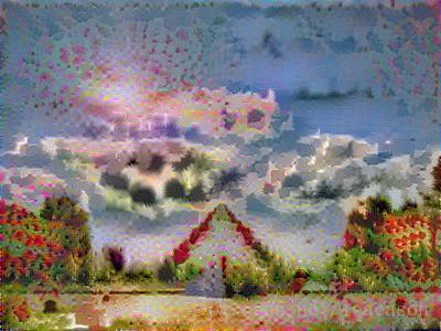
    return generated_image

20次迭代後的圖片：

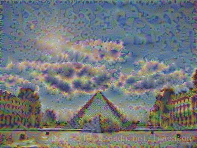
180次迭代後的圖片：

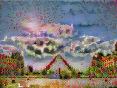
200次迭代後的圖片：