泛化與過擬合

olympval.m

Load the Olympic data and extract the training and validation data

load data/olympics
x = male100(:,1);
t = male100(:,2);
pos = find(x>1979);
% Rescale x for numerical reasons
x = x - x(1);
x = x./4;

valx = x(pos:end);
valt = t(pos:end);
x(pos:end) = [];
t(pos:end) = [];

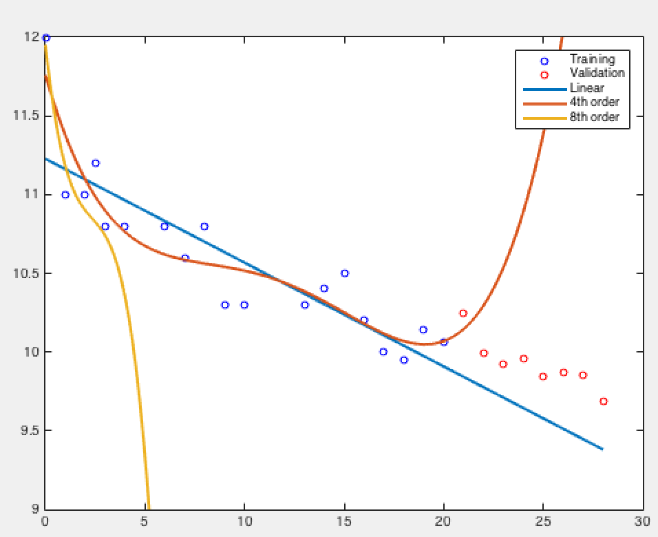
Fit the different models and plot the results

orders = [1 4 8]; %We shall fit models of these orders
% Plot the data
figure(1);hold off
plot(x,t,'bo','markersize',5);
hold all
plot(valx,valt,'ro','markersize',5);
plotx = [min(x):0.01:max(valx)]';
for i = 1:length(orders)
    X = [];
    plotX = [];
    valX = [];
    for k = 0:orders(i)
        X = [X x.^k]
 
;
        valX = [valX valx.^k];
        plotX = [plotX plotx.^k];
    end

    % Compute w
    w = inv(X'*X)*X'*t;
    plot(plotx,plotX*w,'linewidth',2);

    % Compute validation loss
    val_loss(i) = mean((valX*w - valt).^2);
end
ylim([9 12]);
legend('Training','Validation','Linear','4th order','8th order'
 
);

Display the validation losses

for i = 1:length(orders)
 fprintf('\n Model order: %g, Validation loss: %g',...
        orders(i),val_loss(i));
end

Model order: 1, Validation loss: 0.101298
Model order: 4, Validation loss: 4.45706
Model order: 8, Validation loss: 3.72921e+07

cv_demo.m

Generate some data
Generate x between -5 and 5

N = 100;
x = 10*rand(N,1) - 5;
t = 5*x.^3  - x.^2 + x + 150*randn(size(x));
testx = [-5:0.01:5]'; % Large, independent test set
testt = 5*testx.^3 - testx.^2 + testx + 150*randn(size(testx));

Run a cross-validation over model orders

maxorder = 7;
X = [];
testX = [];
K = 10 %K-fold CV
sizes = repmat(floor(N/K),1,K);
sizes(end) = sizes(end) + N - sum(sizes);
csizes = [0 cumsum(sizes)];

% Note that it is often sensible to permute the data objects before
% performing CV.  It is not necessary here as x was created randomly.  If
% it were necessary, the following code would work:
% order = randperm(N);
% x = x(order); Or: X = X(order,:) if it is multi-dimensional.
% t = t(order);

for k = 0:maxorder
    X = [X x.^k];
    testX = [testX testx.^k];
    for fold = 1:K
        % Partition the data
        % foldX contains the data for just one fold
        % trainX contains all other data

        foldX = X(csizes(fold)+1:csizes(fold+1),:);
        trainX = X;
        trainX(csizes(fold)+1:csizes(fold+1),:) = [];
        foldt = t(csizes(fold)+1:csizes(fold+1));
        traint = t;
        traint(csizes(fold)+1:csizes(fold+1)) = [];

        w = inv(trainX'*trainX)*trainX'*traint;
        fold_pred = foldX*w;
        cv_loss(fold,k+1) = mean((fold_pred-foldt).^2);
        ind_pred = testX*w;
        ind_loss(fold,k+1) = mean((ind_pred - testt).^2);
        train_pred = trainX*w;
        train_loss(fold,k+1) = mean((train_pred - traint).^2);
    end
end

K =

10

Plot the results

figure(1);
subplot(311)
plot(0:maxorder,mean(cv_loss,1),'linewidth',2)
xlabel('Model Order');
ylabel('Loss');
title('CV Loss');
subplot(312)
plot(0:maxorder,mean(train_loss,1),'linewidth',2)
xlabel('Model Order');
ylabel('Loss');
title('Train Loss');
subplot(313)
plot(0:maxorder,mean(ind_loss,1),'linewidth',2)
xlabel('Model Order');
ylabel('Loss');
title('Independent Test Loss')

正規化最小二乘法

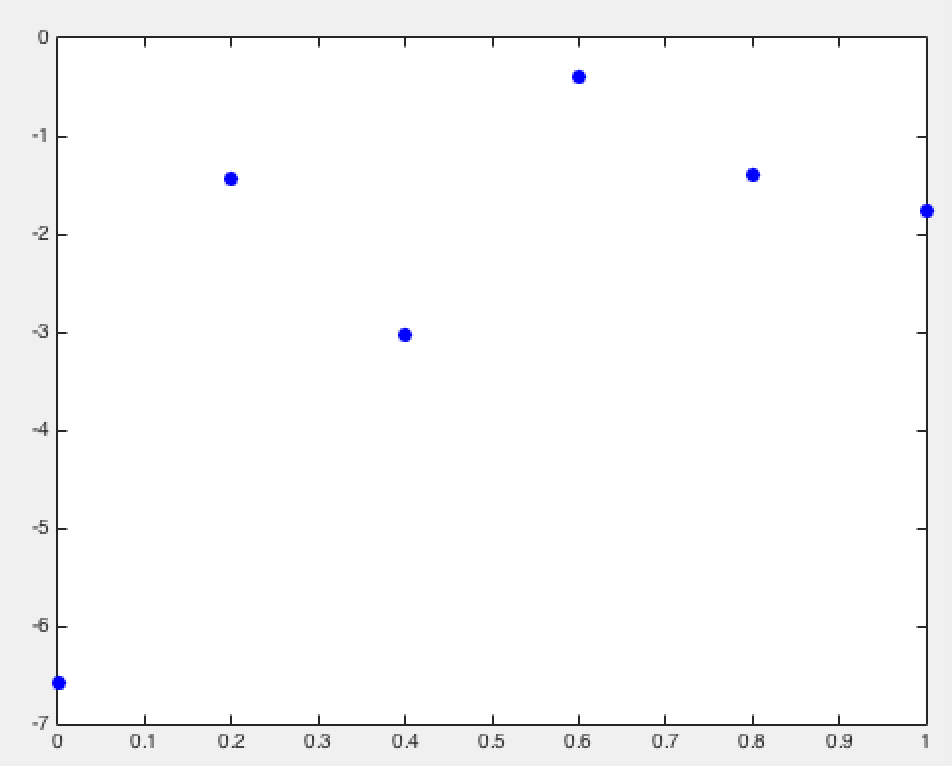
An example of regularised least squares Data is generated from a linear model and then a fifth order polynomial is fitted. The objective (loss) function that is minimisied is

x = [0:0.2:1]';
y = 2*x-3;

Create targets by adding noise

noisevar = 3;
t = y + sqrt(noisevar)*randn(size(x));

Plot the data

plot(x,t,'b.','markersize',25);

Build up the data so that it has up to fifth order terms

plotX = [0:0.01:1]';
X = [];
plotX = [];
for k = 0:5
    X = [X x.^k];
    plotX =[plotX plotx.^k];
end

Fit the model with different values of the regularisation parameter

lam = [0 1e-6 1e-2 1e-1];
for l = 1:length(lam)
    lambda = lam(l);
    N = size(x,1);
    w = inv(X'*X + N*lambda*eye(size(X,2)))*X'*t;
    figure(1);hold off
    plot(x,t,'b.','markersize',20);
    hold on
    plot(testX,TestX*w,'r','linewidth',2)
    xlim([-0.1 1.1])
    xlabel('$x$','interpreter','latex','fontsize',15);
    ylabel('$f(x)$','interpreter','latex','fontsize',15);
    ti = sprintf('$\\lambda = %g$',lambda);
    title(ti,'interpreter','latex','fontsize',20)
end