Numpy快速入門教程(三):SciPy,Matplotlib
首先宣告本篇部落格是本人學習CS231n的學習筆記,分享給大家當作參考。
SciPy
Numpy提供了高效能的多維陣列,以及計算和運算元組的基本工具。SciPy基於Numpy,提供了大量的計算和運算元組的函式,這些函式對於不同型別的科學和工程計算非常有用。
熟悉SciPy的最好方法就是閱讀文件。我們會強調對於本課程有用的部分。
影象操作
SciPy提供了一些操作影象的基本函式。比如,它提供了將影象從硬碟讀入到陣列的函式,也提供了將陣列中資料寫入的硬碟成為影象的函式。下面是一個簡單的例子:
from scipy.misc import imread, imsave, imresize
# Read 可能會報錯顯示沒有安裝相關的科學計算包,所以在此強烈推薦使用Anaconda而不是其他IDE。
Anaconda在python語言外,還集成了numpy、scipy、matplotlib等科學計算包,以及beautiful-soup、requests、lxml等網路相關包。
安裝Anaconda後,基本不再需要費勁地安裝其他第三方庫了。
結果如圖:


MATLAB檔案
函式scipy.io.loadmat和scipy.io.savemat能夠讓你讀和寫MATLAB檔案。具體請檢視文件。
點之間的距離
SciPy定義了一些有用的函式,可以計算集合中點之間的距離。
函式scipy.spatial.distance.pdist能夠計算集合中所有兩點之間的距離:
import numpy as np
from scipy.spatial.distance import pdist, squareform

# Create the following array where each row is a point in 2D space:
# [[0 1]
#  [1 0]
#  [2 0]]
x = np.array([[0, 1], [1, 0], [2, 0]])
print(x)

# Compute the Euclidean distance between all rows of x.
# d[i, j] is the Euclidean distance between x[i, :] and x[j, :],
# and d is the following array:
# [[ 0.          1.41421356  2.23606798]
#  [ 1.41421356  0.          1.        ]
#  [ 2.23606798  1.          0.        ]]
d = squareform(pdist(x, 'euclidean'))
print(d)具體細節請閱讀文件。
函式scipy.spatial.distance.cdist可以計算不同集合中點的距離,具體請檢視文件。
Matplotlib
Matplotlib是一個作相簿。這裡簡要介紹matplotlib.pyplot模組,功能和MATLAB的作圖功能類似。
繪圖
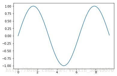
matplotlib庫中最重要的函式是Plot。該函式允許你做出2D圖形,如下:
import numpy as np
import matplotlib.pyplot as plt

# Compute the x and y coordinates for points on a sine curve
x = np.arange(0, 3 * np.pi, 0.1)
y = np.sin(x)

# Plot the points using matplotlib
plt.plot(x, y)
plt.show()  # You must call plt.show() to make graphics appear.
結果如下圖:
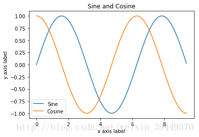
只需要少量工作,就可以一次畫不同的線,加上標籤,座標軸標誌等。
import numpy as np
import matplotlib.pyplot as plt

# Compute the x and y coordinates for points on sine and cosine curves
x = np.arange(0, 3 * np.pi, 0.1)
y_sin = np.sin(x)
y_cos = np.cos(x)

# Plot the points using matplotlib
plt.plot(x, y_sin)
plt.plot(x, y_cos)
plt.xlabel('x axis label')
plt.ylabel('y axis label')
plt.title('Sine and Cosine')
plt.legend(['Sine', 'Cosine'])
plt.show()
結果圖如下:
可以在文件中閱讀更多關於plot的內容。
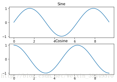
繪製多個影象
可以使用subplot函式來在一幅圖中畫不同的東西:
import numpy as np
import matplotlib.pyplot as plt

# Compute the x and y coordinates for points on sine and cosine curves
x = np.arange(0, 3 * np.pi, 0.1)
y_sin = np.sin(x)
y_cos = np.cos(x)

# Set up a subplot grid that has height 2 and width 1,
# and set the first such subplot as active.
plt.subplot(2, 1, 1)

# Make the first plot
plt.plot(x, y_sin)
plt.title('Sine')

# Set the second subplot as active, and make the second plot.
plt.subplot(2, 1, 2)
plt.plot(x, y_cos)
plt.title('Cosine')

# Show the figure.
plt.show()
結果如下圖:
關於subplot的更多細節,可以閱讀文件。
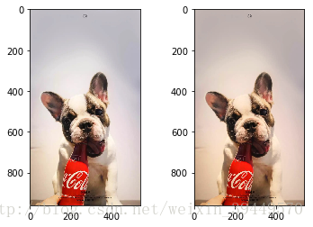
影象
你可以使用imshow函式來顯示影象,如下所示:
import numpy as np
from scipy.misc import imread, imresize
import matplotlib.pyplot as plt

img = imread('dog.jpg')
img_tinted = img * [1, 0.95, 0.9]

# Show the original image
plt.subplot(1, 2, 1)
plt.imshow(img)

# Show the tinted image
plt.subplot(1, 2, 2)

# A slight gotcha with imshow is that it might give strange results
# if presented with data that is not uint8. To work around this, we
# explicitly cast the image to uint8 before displaying it.
plt.imshow(np.uint8(img_tinted))
plt.show()
結果如下圖: