一、實驗題目

1.      拍攝的含有正弦波（ref1.bmp, obj1.bmp）和三角波條紋(T20r1.bmp, T20o1.bmp)投影影象

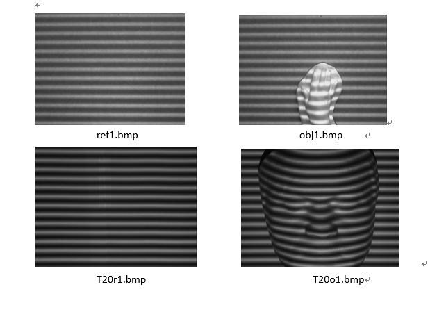
2.      對影象進行濾波去除噪聲，噪聲來源未知，濾波方法和濾波器可參考課程中的內容

3.      選擇最優的濾波器和濾波器引數，要求濾波後的效果：能夠基本恢復原來正弦波或三角波的形狀

4.      要求提交實驗報告作為平時成績，佔總成績50%，包括原始碼和濾波前後的截圖，濾波器設計和使用的思路，評價，分析等。

例如：

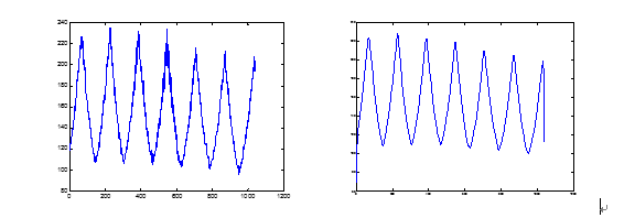
影象中一個y截面濾波前三角波波形（左），濾波後三角波波形（右）

注：濾波三角波要防止三角波頂底部的特徵點因為濾波後變得圓滑平緩

二、實驗程式碼：

2.1 濾波器函式filt.m

%均值濾波
subplot(1,2,1);
img=imread('obj1.bmp');
imshow(img);
xlabel('(1) 原始影象');
A=fspecial('average',[7,7]);%3x3均值濾波
m1=imfilter(img,A);
subplot(1,2,2),imshow(m1,[]);
xlabel('(2) 1次7x7均值濾波');
imwrite(m1,'obj1_1_7x7avgfilt.bmp');

%中值濾波
subplot(1,2,1);
img=imread('obj1.bmp');
imshow(img);
xlabel('(1) 原始影象');
m1=medfilt2(img,[3,3]);
subplot(1,2,2),imshow(m1,[]);
xlabel('(2) 1次3x3中值濾波');
imwrite(m1,'obj1_1_3x3medfilt.bmp');

%維納濾波
subplot(1,2,1);
img=imread('obj1.bmp');
imshow(img);
xlabel('(1) 原始影象');
m1=wiener2(img, [3 3]);%3x3自適應維納濾波
subplot(1,2,2),imshow(m1,[]);
xlabel('(2) 1次3x3維納濾波');
imwrite(m1,'obj1_1_3x3_wienerfilt.bmp');

%高斯濾波 
subplot(1,2,1);
img=imread('T20r1.bmp');
imshow(img);
xlabel('(1) 原始影象');
%k=input('請輸入高斯濾波器的均值/n');  
%n=input('請輸入高斯濾波器的方差/n');  
A1=fspecial('gaussian',3,5);      %生成高斯序列  
m1=filter2(A1,img)/255;             %用生成的高斯序列進行濾波
subplot(1,2,2),imshow(m1,[]);
xlabel('(2) 1次均值為3方差為0.1的高斯濾波');
imwrite(m1,'T20r1_3_50_gaussianfilt.bmp');
 

%濾波前後對比
figure;
subplot(2,1,1);
h=imread('T20r1_3_50_gaussianfilt.bmp');
[m n]=size(h);
s=1;
arr=[];
    for i=1:m
        for j=1:n       
            if(j==50)
            arr(s)=h(i,j,1);
            s=s+1; 
           end
        end         
    end
plot(arr);

subplot(2,1,2);
h2=imread('obj1_1_3x3avgfilt.bmp');
[m n]=size(h2);
s=1;
arr=[];
    for i=1:m
        for j=1:n       
            if(j==50)
            arr(s)=h2(i,j,1);
            s=s+1; 
           end
        end         
    end
plot(arr);
 

% Demo to calculate PSNR of a gray scale image.
% http://en.wikipedia.org/wiki/PSNR
% Clean up.
clc;    % Clear the command window.
close all;  % Close all figures (except those of imtool.)
clear;  % Erase all existing variables. Or clearvars if you want.
workspace;  % Make sure the workspace panel is showing.
format long g;
format compact;
fontSize = 20;

%------ GET DEMO IMAGES ----------------------------------------------------------
% Read in a standard MATLAB gray scale demo image.
refImage = imread('T20r1_3_50_gaussianfilt.bmp');

% Display the first image.
subplot(3, 2, 1);
imshow(refImage, []);
title('After filt ref Image', 'FontSize', fontSize);

% Cut ref Image 從上到下 從左到右
refImage_cut = refImage(20:1000,20:150);
[rows columns] = size(refImage_cut);
subplot(3, 2, 2);
imshow(refImage_cut, []);
title('Cut after filt ref Image', 'FontSize', fontSize);

% Get a second image by adding noise to the first image.
%noisyImage = imnoise(grayImage, 'gaussian', 0, 0.003);

% Read the second image
objImage = imread('T20o1_3_50_gaussianfilt.bmp');
% Display the second image.
subplot(3, 2, 3);
imshow(objImage, []);
title('After filt obj Image', 'FontSize', fontSize);

% Cut obj Image 從上到下 從左到右
objImage_cut = objImage(20:1000,20:150);
subplot(3, 2, 4);
imshow(objImage_cut, []);
title('Cut After filt obj Image', 'FontSize', fontSize);

%------ PSNR CALCULATION ----------------------------------------------------------
% Now we have our two images and we can calculate the PSNR.
% First, calculate the "square error" image.
% Make sure they're cast to floating point so that we can get negative differences.
% Otherwise two uint8's that should subtract to give a negative number
% would get clipped to zero and not be negative.
squaredErrorImage = (double(refImage_cut) - double(objImage_cut)) .^ 2;
% Display the squared error image.
subplot(3, 2, 5);
imshow(squaredErrorImage, []);
title('Squared Error Image', 'FontSize', fontSize);
% Sum the Squared Image and divide by the number of elements
% to get the Mean Squared Error.  It will be a scalar (a single number).
mse = sum(sum(squaredErrorImage)) / (rows * columns);
rmse = sqrt(mse);
% Calculate PSNR (Peak Signal to Noise Ratio) from the MSE according to the formula.
PSNR = 10 * log10( 256^2 / mse);
% Alert user of the answer.
message = sprintf('The mean square error is %.2f.\nThe PSNR = %.2f', rmse, PSNR);
msgbox(message);