Testing while documenting

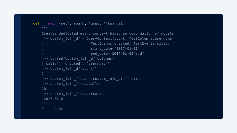
All critical paths of the code are covered with Integration Tests using Python Doctest framework, enabling up-to-date and accurate usage documentation for each team that uses the data science platform. The tests allow us to have the following style of documentation, which is validated daily:

Spark and Jupyter: working together

Spark is commonly used in the cloud. And in cloud-based deployments, it is relatively easy for data scientists to spin up clusters for their individual needs. But since we were on premise, we were working with a single shared cluster, meaning it would take a relatively long time to add new servers to our data center.

Therefore, we had to optimize for as many concurrent analyses as possible to run on the existing hardware. To achieve this, we had to apply very specific configurations, and then optimize these configurations to suit our own situation.

Executor cores and caching
Initially we allocated a static number (5–10) of executor cores to each notebook . This worked well, until the number of people using the platform doubled.

spark.dynamicAllocation.enabled=true
spark.dynamicAllocation.maxExecutors=7
spark.dynamicAllocation.minExecutors=1

This worked well for a period of time, until people actively started caching their dataframes. This means the dataframes are stored in the memory of the executor. By default, executors with cached data are not subject to deallocation, so each notebook would effectively stay at their maxExecutors, rendering dynamic (de)allocation useless. At that time this option was under-documented. After trial and error we figured out that within our organization, five minutes of inactivity is the most optimal period to shut off access to compute resources:

spark.dynamicAllocation.cachedExecutorIdleTimeout=5m

Killer chatbot
Initially our idea was that each data scientist would stop their notebooks/drivers to release resources back to cluster. In practice, however, people sometimes forgot or delayed this. Since human-based processes don’t work until they are automated, we implemented a kill script that runs at regular intervals to notify data scientists, via chatbot, that their notebooks were forcefully shut down due to 30 minutes of inactivity:

Broadcast join
A significant performance benefit came from increasing the value of:

spark.sql.autoBroadcastJoinThreshold=256m

This helped optimize large joins, from the default of 10MB to 256MB. In fact, we started to see performance increases between 200% to 700%, depending on amount of joined partitions and type of the query.

The optimal value of this setting can be determined by caching and counting a dataframe and then checking the value in the “Storage” tab within the Spark UI. The best practice is also to force broadcasts of small-enough dataframes with sizes up to few hundred megabytes within the code as well:

df.join(broadcast(df2), df.id == df2.id)

The other settings that helped our multi-tenant setup were:

# we had to tune for unstable networks and overloaded servers

spark.port.maxRetries=30
spark.network.timeout=500
spark.rpc.numRetries=10

# we sacrificed a bit of speed for the sake of data consistency

spark.speculation=false

Persistence
From a storage perspective, we selected the default columnar-based format, Apache Parquet, and partitioned it (mostly) by date. After a while, we also started bucketing certain datasets as second level partitioning. (Rule of thumb — use bucketing only if query performance cannot be optimized by picking the right data structure and using correct broadcasts.)

For the first few months we worked with simple date-partitioned directories containing parquet files. Then we switched to Hive Metastore provided by spark-thriftserver, giving us the ability to expose certain datasets to our business users through Looker.

Merge schema
In the beginning we treated our Parquet datasets as semi-structured and had:

spark.sql.parquet.mergeSchema=true 

After six months we switched mergeSchema to false, as with schema-less flexibility there is a performance penalty upon cold notebook start. We wanted to finally migrate to a proper metastore.

Spoink — Lightweight Spark-focused data pipeline

In the beginning, data was created through notebooks, and scheduled in the background by cron. This was a temporary hack to get the ball rolling, but did not provide sufficient functionality for the long term.

For this, we needed a standardized tool that was simple, had an error recovery mode, supported specific order execution, and idempotent execution. Code footprint and quality assurance for our data pipelines were also key considerations.

Initially, we looked at tools such as Airflow and Luigi. However these are primarily focused on spinning up dedicated Spark clusters in the cloud. They would have required hundreds of external dependencies to be compiled by our infrastructure team to go live.

So instead, we took the best concepts from existing tools — checkpointing, cross-dependent execution, and immutable data — and created our own orchestrator/scheduler, that worked primarily with single shared Spark cluster. We called it Spoink, in order to be “logical” and “consistent” with the big data ecosystem.

Within the Spoink framework, every table is called a DataSource. It requires a function to create a Spark dataframe and registration in specific scheduled interval. We are also required to specify which metastore table to be populated, and how data would be partitioned:

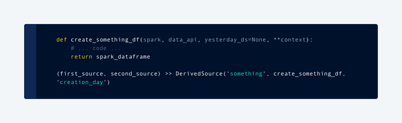
With this setup, it became very easy to develop and test ETL functionality within Jupyter notebooks with live data. It also meant we were able to repeat this process back in time just by invoking the same function for previous days.

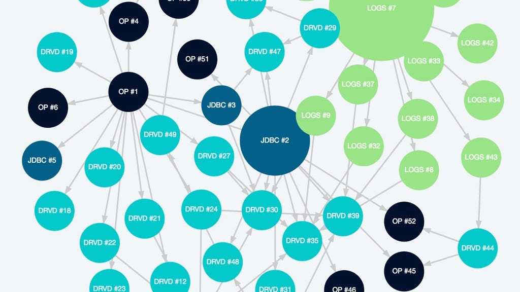
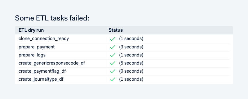
We have a few top-level types of data sources, like LogSource, PostgreSource and DerivedSource. The core data science platform team owns most of the log and postgres-based sources, and data scientists have almost full freedom to create and modify DerivedSources. We forced every datasource to be pure functions, which enables us to dry-run it multiple times per day and quickly see things that may break production ETL processing:

Data API

Every data team has its own structure and reusable components. In the pre-Spark era, we had a bunch of R scripts — basically a collection of SQL queries. This created some confusion in consistently computing business-important metrics such as payment authorization or chargeback rates.

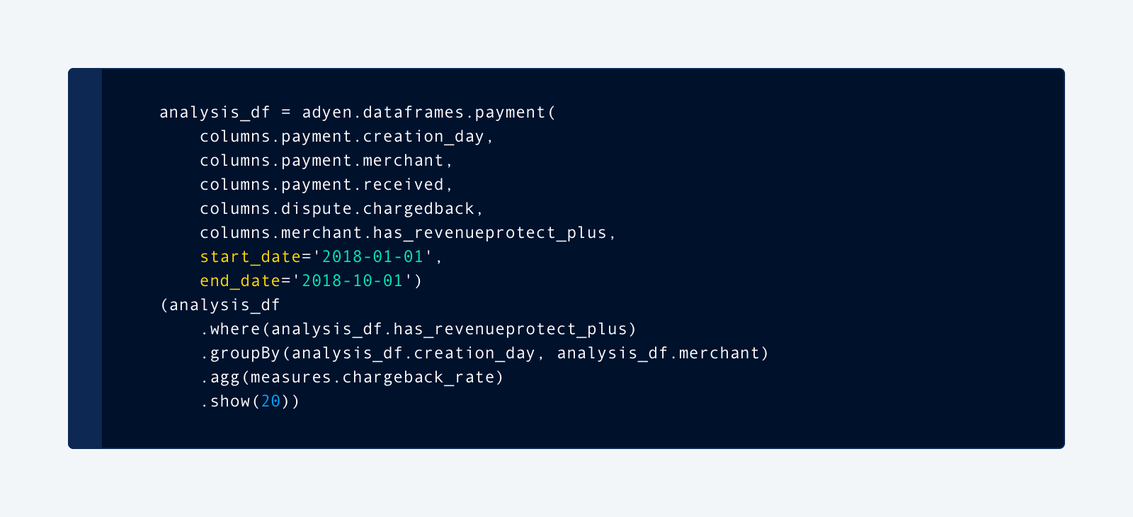
Following a very positive experience with Looker view modeling, we were excited to have something like that for our ML: a place in code, where we define certain views on data, how it’s joined with other datasets, and metrics derived from it. This was preferable to hard-coding dataframes every time when needed, and having to know which tables and possible dimensions/measures exist.

Here’s an example that creates our interactive chargeback rate report (and hides the complexity of joining all the underlying sources):

Beta flow

%adyen_beta (a.k.a. JRebel for Jupyter/Spark) gives tremendous benefits to the quality of Spark code and workflows in general. It allows us to update code in notebook runtime directly, by pushing to the Git master branch without restarting the notebook. Here’s how it works: