
deep learning 自學習網路的Softmax分類器
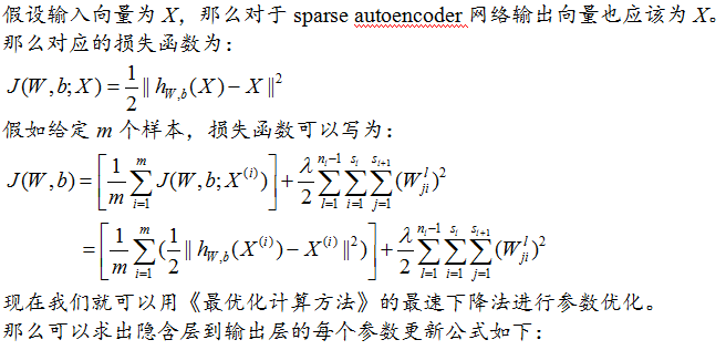
這一節我將跳過KNN分類器,因為KNN分類器分類時間效率太低,這一節講Sparse autoencoder + softmax分類器。首先普及一下Sparse autoencoder網路,Sparse autoencoder可以看成一個3層神經網路,但是輸入的數目和輸出的個數相等。Sparse autoencoder的作用是提取特徵,和PCA的功能有點類似,那麼Sparse autoencoder是如何提取特徵向量的呢?其實提取的特徵就是隱含層的輸出,首先來講sparse autoencoder模型的圖例如下:
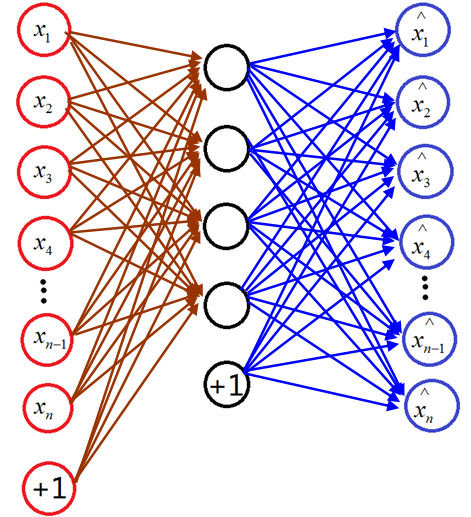
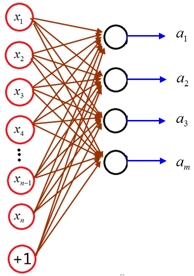
我們去掉輸出層以後,隱含層的值就是我們需要求的特徵值,假如有n個輸入,隱含層有m
 就是輸出特徵值,然後再接上softmax分類器就形成了sparse autoencoder softmax分類器。特徵值表示如下圖:
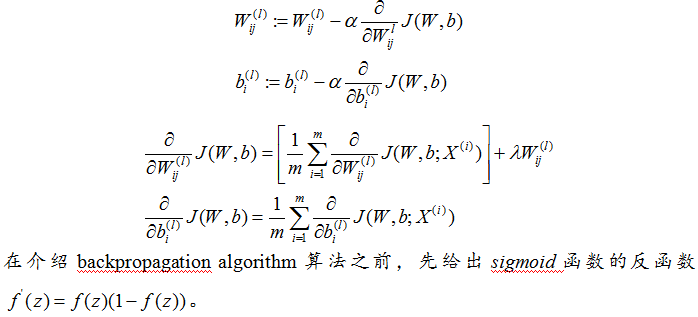
下面分別講Sparse autoencoder softmax分類器每一步:
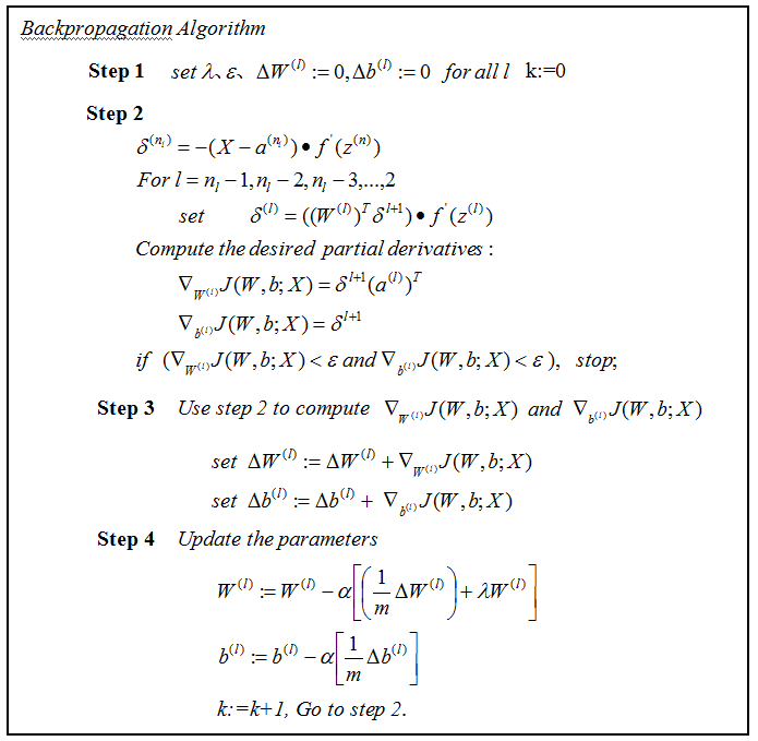
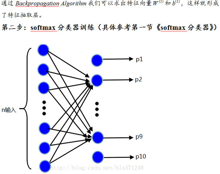
第一步:Sparse autoencoder
神經網路分為前饋和後饋
前饋網路
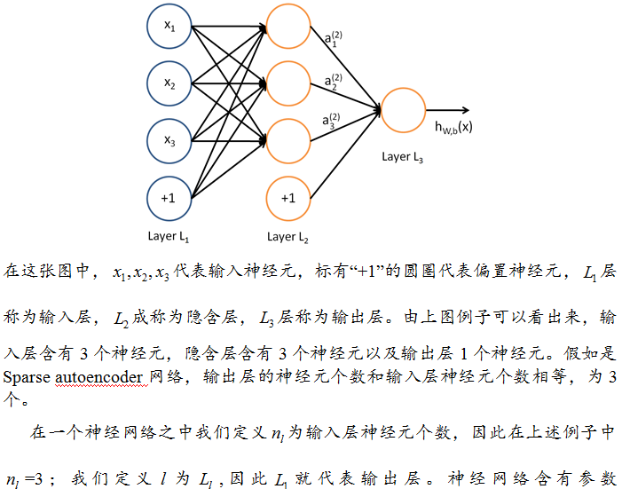
一個神經網路是通過很多簡單的神經元構成,下面是一個簡單的神經網路。
後饋網路
softmax分類器第一節有講,sparse autoencoder網路訓練用的是SD法,softmax分類器訓練用的L-BFGS,具體可以參見《最優化計算方法》板塊。
實驗與結果
MNIST數字識別庫的圖片是28×28大小尺寸,假如隱含層有200個神經元,那麼在sparse autoencoder網路中就含有(784+1)*(200)+(200+1)*784=314584個引數。那麼原來的softmax分類器需要784*10=7840個引數,現在經過特徵抽取後只需要200*10=2000個引數。可以提取出這些資料的權值,權值轉換成圖片顯示如下:

(1)sparse autoencoder網路損失函式隨著迭代次數的曲線
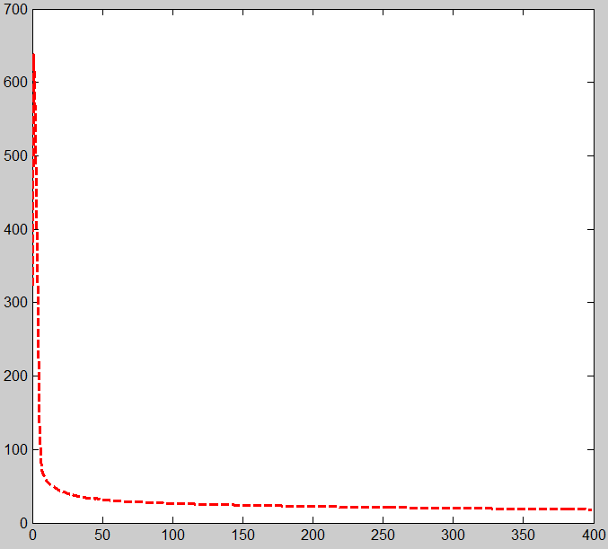
最後通過softmax分類器可以得到識別率為97.21%,比直接用softmax分類器分類識別率高,直接softmax分類器的識別率為92.67%。具體程式碼見資源!
sparseautoencoder_softmax.m
%% ======================================================================
%  STEP 0: Here we provide the relevant parameters values that will
%  allow your sparse autoencoder to get good filters; you do not need to
%  change the parameters below.

inputSize  = 28 * 28;
numLabels  = 10;
hiddenSize = 200;
sparsityParam = 0.1; % desired average activation of the hidden units.
% (This was denoted by the Greek alphabet rho, which looks like a lower-case "p",
%  in the lecture notes).
lambda = 3e-3;       % weight decay parameter
beta = 3;            % weight of sparsity penalty term
maxIter = 450;
numClasses = 10;     % Number of classes (MNIST images fall into 10 classes)
lambda = 1e-4; % Weight decay parameter
itera_num=120;
Learningrate=0.6;
a=1;roi=0.5;c=0.6;m=10;
%% ======================================================================
%  STEP 1: Load data from the MNIST database
%
%  This loads our training and test data from the MNIST database files.
%  We have sorted the data for you in this so that you will not have to
%  change it.
% Load MNIST database files
images=loadMNISTImages('train-images.idx3-ubyte');
labels=loadMNISTLabels('train-labels.idx1-ubyte');
labels(labels==0) = 10;
%% ======================================================================
%  STEP 2: Train the sparse autoencoder
%  This trains the sparse autoencoder on the unlabeled training
%  images.
%  Randomly initialize the parameters
theta = initializeParameters(hiddenSize, inputSize);
%% sparseAutoencoder
W1 = reshape(theta(1:hiddenSize*inputSize), hiddenSize, inputSize);
W2 = reshape(theta(hiddenSize*inputSize+1:2*hiddenSize*inputSize), inputSize, hiddenSize);
b1 = theta(2*hiddenSize*inputSize+1:2*hiddenSize*inputSize+hiddenSize);
b2 = theta(2*hiddenSize*inputSize+hiddenSize+1:end);
% Cost and gradient variables (your code needs to compute these values).
% Here, we initialize them to zeros.

W1grad = zeros(size(W1));
W2grad = zeros(size(W2));
b1grad = zeros(size(b1));
b2grad = zeros(size(b2));
%%
Jcost = 0;%直接誤差
Jweight = 0;%權值懲罰
Jsparse = 0;%稀疏性懲罰
[n m] = size(images);%m為樣本的個數,n為樣本的特徵數
fprintf('%10s %10s','Iteration','cost','Accuracy');
fprintf('\n');
for i=1:maxIter
    %前向演算法計算各神經網路節點的線性組合值和active值
    z2 = W1*images+repmat(b1,1,m);%注意這裡一定要將b1向量複製擴充套件成m列的矩陣
    a2 = sigmoid(z2);
    z3 = W2*a2+repmat(b2,1,m);
    a3 = sigmoid(z3);
    % 計算預測產生的誤差
    Jcost = (0.5/m)*sum(sum((a3-images).^2));

    %計算權值懲罰項
    Jweight = (1/2)*(sum(sum(W1.^2))+sum(sum(W2.^2)));

    %計算稀釋性規則項
    rho = (1/m).*sum(a2,2);%求出第一個隱含層的平均值向量
    Jsparse = sum(sparsityParam.*log(sparsityParam./rho)+(1-sparsityParam).*log((1-sparsityParam)./(1-rho))); %損失函式的總表示式
    cost(i) = Jcost+lambda*Jweight+beta*Jsparse;
    %反向演算法求出每個節點的誤差值
    d3 = -(images-a3).*sigmoidInv(z3);
    sterm = beta*(-sparsityParam./rho+(1-sparsityParam)./(1-rho));%因為加入了稀疏規則項,所以
    %計算偏導時需要引入該項
    d2 = (W2'*d3+repmat(sterm,1,m)).*sigmoidInv(z2);
    %計算W1grad
    W1grad = W1grad+d2*images';
    W1grad = (1/m)*W1grad+lambda*W1;
    %計算W2grad
    W2grad = W2grad+d3*a2';
    W2grad = (1/m).*W2grad+lambda*W2;
    %計算b1grad
    b1grad = b1grad+sum(d2,2);
    b1grad = (1/m)*b1grad;%注意b的偏導是一個向量,所以這裡應該把每一行的值累加起來
    %計算b2grad
    b2grad = b2grad+sum(d3,2);
    b2grad = (1/m)*b2grad;
    W1=W1-Learningrate*W1grad;
    W2=W2-Learningrate*W2grad;
    b1=b1-Learningrate*b1grad;
    b2=b2-Learningrate*b2grad;
    fprintf('%5d     %13.4e  \n',i,cost(i));
end
%-------------------------------------------------------------------

display_network(W1');
figure
plot(0:499, cost(1:500),'r--','LineWidth', 2);
%================================================
%STEP 3: 訓練Softmax分類器
activation  = sigmoid(W1*images+repmat(b1,[1,size(images,2)]));
theta = 0.005 * randn(numClasses * hiddenSize, 1);%輸入的是一個列向量
% Randomly initialise theta
theta = reshape(theta, numClasses, hiddenSize);%將輸入的引數列向量變成一個矩陣
inputData = activation;
numCases = size(inputData, 2);%輸入樣本的個數
groundTruth = full(sparse(labels, 1:numCases, 1));%這裡sparse是生成一個稀疏矩陣,該矩陣中的值都是第三個值1
%稀疏矩陣的小標由labels和1:numCases對應值構成

thetagrad = zeros(numClasses, hiddenSize);

p = weight(theta,inputData);
Jcost(1) = -1/numCases * groundTruth(:)' * log(p(:)) + lambda/2 * sum(theta(:) .^ 2);
thetagrad = -1/numCases * (groundTruth - p) * inputData' + lambda * theta;
B=eye(numClasses);
H=-inv(B);
d1=H*thetagrad;
theta_new=theta+a*d1;
theta_old=theta;
fprintf('%10s %10s %15s %15s %15s','Iteration','cost','Accuracy');
fprintf('\n');
%% Training
for i=2:itera_num %計算出某個學習速率alpha下迭代itera_num次數後的引數
    a=1;
    theta_new=reshape(theta_new, numClasses,hiddenSize);
    theta_old=reshape(theta_old,numClasses,hiddenSize);
    p=weight(theta_new,inputData);
    Mp=weight(theta_old,inputData);
    Jcost(i)=-1/numCases * groundTruth(:)' * log(p(:)) + lambda/2 * sum(theta_new(:) .^ 2);
    thetagrad_new = -1/numCases * (groundTruth - p) * inputData' + lambda * theta_new;
    thetagrad_old = -1/numCases * (groundTruth - Mp) * inputData' + lambda * theta_old;
    thetagrad_new=reshape(thetagrad_new,numClasses*hiddenSize,1);
    thetagrad_old=reshape(thetagrad_old,numClasses*hiddenSize,1);
    theta_new=reshape(theta_new,numClasses*hiddenSize,1);
    theta_old=reshape(theta_old,numClasses*hiddenSize,1);
    M(:,i-1)=thetagrad_new-thetagrad_old;
    BB(:,i-1)=theta_new-theta_old;
    roiJ(i-1)=1/(M(:,i-1)'*BB(:,i-1));
    gamma=(BB(:,i-1)'*M(:,i-1))/(M(:,i-1)'*M(:,i-1));
    HK=gamma*eye(hiddenSize*numClasses);
    r=lbfgsloop(i,m,HK,BB,M,roiJ,thetagrad_new);
    d=-r;
    d=reshape(d,numClasses,hiddenSize);
    theta_new=reshape(theta_new,numClasses,hiddenSize);
    theta_old=theta_new;
    theta_new = theta_new + a*d;
    %% test the accuracy
    fprintf('%5d     %13.4e \n',i,Jcost(i));
end
plot(0:119, Jcost(1:120),'r-o','LineWidth', 2);
testData = loadMNISTImages('t10k-images.idx3-ubyte');
labels1 = loadMNISTLabels('t10k-labels.idx1-ubyte');
labels1(labels1==0) = 10;

test  = sigmoid(W1*testData+repmat(b1,[1,size(testData,2)]));
inputDatatest = test;
pred = zeros(1, size(inputDatatest, 2));
[nop,pred]=max(theta_new*inputDatatest);
acc = mean(labels1(:) == pred(:));
acc=acc * 100
========================================================================================
第三節:從自我學習到深層網路學習
========================================================================================
懷柔風光