
tensorflow學習筆記(七):YOLO v1學習筆記
1、網路結構
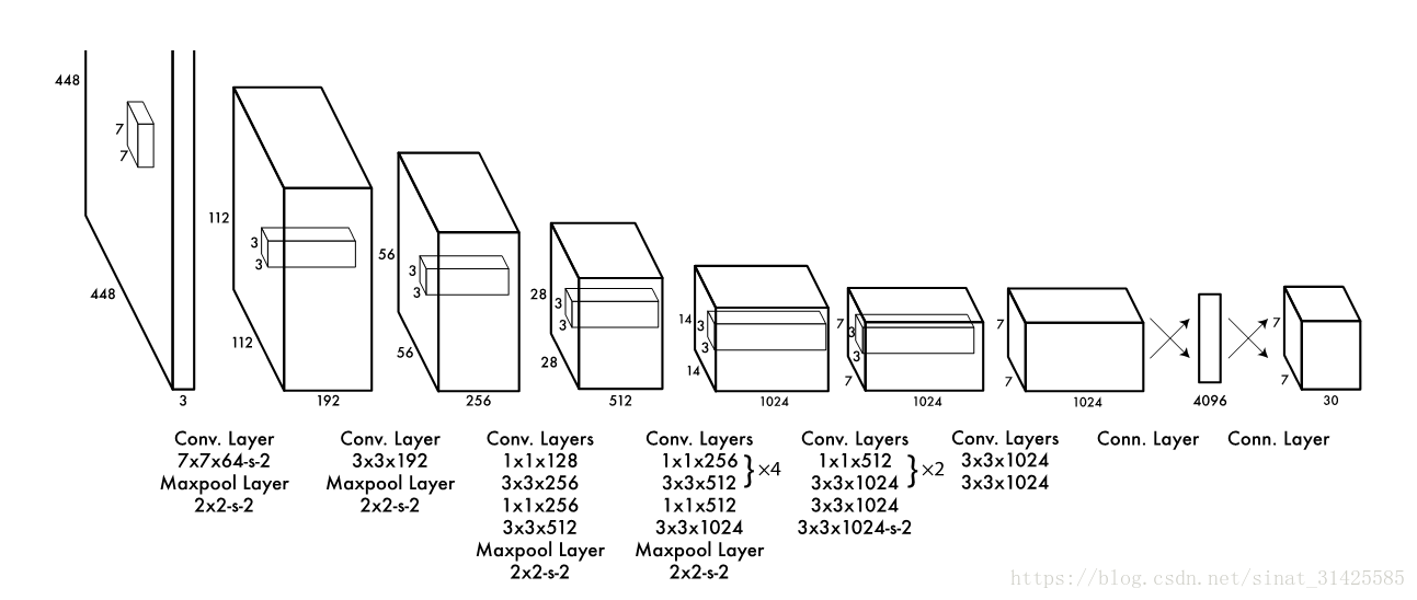
這裡,所有卷積操作都是'SAME'方式,所以以步長為1的卷積操作過程中,不會影響輸出feature map的width和height,feature map大小變化源自於卷積步長和pooling池化操作,而這兩種因素都保留了feature map中元素與輸入影象塊之間的相對位置關係。因此,尺寸為448x448大小影象,經過一系列卷積層、下采樣層之後,最終輸出7x7大小feature map,feature map中每個cell對應於輸入影象中影象塊大小為:448/7 = 64,相當於將輸入影象分割成7x7個影象塊,就可以將影象與輸出feature map對應起來,但是,由於網路的輸入從224x224縮放到448x448,所以,實際上影象塊大小為32x32,這裡對應於論文中說的將影象分成SxS個格子。
構建網路的程式碼為:
    def build_network(self, images, keep_prob=0.5, is_training=True, scope='yolo'):
        with tf.variable_scope(scope):
            with slim.arg_scope([slim.conv2d, slim.fully_connected],
                                activation_fn=leaky_relu(self.alpha),
                                weights_initializer=tf.truncated_normal_initializer(0.0, 0.01),
                                weights_regularizer=slim.l2_regularizer(0.0005)):
                # padding:上下左右、上下左右...
                net = tf.pad(images, np.array([[0, 0], [3, 3], [3, 3], [0, 0]]), name='pad_1')
                # 經過padding之後,相當於'SAME'方式的conv
                # c = 64, f = 7, s = 2   ==> 64 x 224 x 224
                net = slim.conv2d(net, 64, 7, 2, padding='VALID', scope='conv_2')
                # max-pooling
                # f = 2, c = 2, p = 'SAME' ==> 64 x 112 x 112
                net = slim.max_pool2d(net, 2, padding='SAME', scope='pool_3')

                # c = 192, f = 3, s = 1    ==> 192 x 112 x  112
                net = slim.conv2d(net, 192, 3, scope='conv_4')
                # max-pooling
                # f = 2, c = 2, p = 'SAME' ==> 192 x 56 x 56
                net = slim.max_pool2d(net, 2, padding='SAME', scope='pool_5')

                # 預設padding為'SAME'
                # c = 128, f = 1, s = 1   ==> 128 x 56 x 56
                net = slim.conv2d(net, 128, 1, scope='conv_6')
                # c = 256, f = 3, s = 1   ==> 256 x 56 x 56
                net = slim.conv2d(net, 256, 3, scope='conv_7')
                # c = 256, f = 1, s = 1   ==> 256 x 56 x 56
                net = slim.conv2d(net, 256, 1, scope='conv_8')
                # c = 512, f = 3, s = 1   ==> 512 x 56 x 56
                net = slim.conv2d(net, 512, 3, scope='conv_9')
                # f = 2, s = 2  ==> 512 x 28 x 28
                net = slim.max_pool2d(net, 2, padding='SAME', scope='pool_10')


                # c = 256, f = 1, s = 1   ==> 256 x 28 x 28
                net = slim.conv2d(net, 256, 1, scope='conv_11')
                # c = 512, f = 3, s = 1, ==> 512 x 28 x 28
                net = slim.conv2d(net, 512, 3, scope='conv_12')
                # c = 256, f = 1, s = 1, ==> 256 x 28 x 28
                net = slim.conv2d(net, 256, 1, scope='conv_13')
                # c = 512, f = 3, s = 1, ==> 512 x 28 x 28
                net = slim.conv2d(net, 512, 3, scope='conv_14')
                # c = 256, f = 1, s = 1, ==> 256 x 28 x 28
                net = slim.conv2d(net, 256, 1, scope='conv_15')
                # c = 512, f = 3, s = 1, ==> 512 x 28 x 28
                net = slim.conv2d(net, 512, 3, scope='conv_16')
                # c = 256, f = 1, s = 1, ==> 256 x 28 x 28
                net = slim.conv2d(net, 256, 1, scope='conv_17')
                # c = 512, f = 3, s = 1, ==> 512 x 28 x 28
                net = slim.conv2d(net, 512, 3, scope='conv_18')
                # c = 512, f = 1, s = 1, ==> 512 x 28 x 28
                net = slim.conv2d(net, 512, 1, scope='conv_19')
                # c = 1024, f = 3, s = 1, ==> 1024 x 28 x 28
                net = slim.conv2d(net, 1024, 3, scope='conv_20')
                # f = 2, s = 2,   ==> 1024 x 14 x 14
                net = slim.max_pool2d(net, 2, padding='SAME', scope='pool_21')

                # c = 512, f = 1, s = 1, ==> 512 x 14 x 14
                net = slim.conv2d(net, 512, 1, scope='conv_22')
                # c = 1024, f = 3, s = 1, ==> 1024 x 14 x 14
                net = slim.conv2d(net, 1024, 3, scope='conv_23')
                # c = 512, f = 1, s = 1, ==> 512 x 14 x 14
                net = slim.conv2d(net, 512, 1, scope='conv_24')
                # c = 1024, f = 3, s = 1, ==> 1024 x 14 x 14
                net = slim.conv2d(net, 1024, 3, scope='conv_25')
                # c = 1024, f = 3, s = 1, ==> 1024 x 14 x 14
                net = slim.conv2d(net, 1024, 3, scope='conv_26')
                # 相當於padding = 'SAME'的conv
                net = tf.pad(net, np.array([[0, 0], [1, 1], [1, 1], [0, 0]]), name='pad_27')
                # c = 1024, f = 3, s = 2  ==> 1024 x 7 x 7
                net = slim.conv2d(net, 1024, 3, 2, padding='VALID', scope='conv_28')
                # c = 1024, f = 3, s = 1, ==> 1024 x 7 x 7
                net = slim.conv2d(net, 1024, 3, scope='conv_29')
                # c = 1024, f = 3, s = 1, ==> 1024 x 7 x 7
                net = slim.conv2d(net, 1024, 3, scope='conv_30')
                # ==> 7 x 7 x 1024
                net = tf.transpose(net, [0, 3, 1, 2], name='trans_31')
                net = slim.flatten(net, scope='flat_32')
                net = slim.fully_connected(net, 512, scope='fc_33')
                net = slim.fully_connected(net, 4096, scope='fc_34')
                net = slim.dropout(net, keep_prob=keep_prob, is_training=is_training, scope='dropout_35')
                net = slim.fully_connected(net, self.output_size, activation_fn=None, scope='fc_36')
        return net
2、輸出7x7x30
YOLO最後輸出的7x7x30中,7x7表示最後輸出feature map大小,每一個位置對應於輸入影象的一個cell,如圖2所示。

圖2 cell對應第一個box資訊(摘自deepsystems.io)
每個cell對應於一個1x30的向量,前面10位對應於位置及置信度資訊,由於每個cell對應兩個box,而每個box對應於一個(x, y, w, h, c),因此當前cell對應的第一個box資訊如圖2所示,當前cell對應第二個box資訊如圖3所示。

圖3 cell對應第二個box資訊(摘自deepsystems.io)
後面20位對應類別資訊,是對於類別資訊的編碼,每個cell,對應於每個box都有一個類別編碼值,如圖4和5所示。

圖 4 box1的類別資訊編碼(摘自deepsystems.io)

圖5 box2的類別資訊編碼(摘自deepsystems.io)
因此,7x7個cell對應於49x2=98個20x1的類別資訊,如圖6所示:
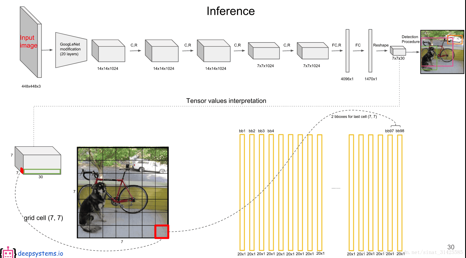
圖6 7x7個cell對應的類別資訊(摘自deepsystems.io)
3、檢測過程
如圖7所示,首先,按照box的得分score(if score < threshold1(0.2), then Set score to zero)判斷當前box中是否存在目標物體;然後,對box的得分score,按照從大到小的順序進行排序;其次,採用NMS(非極大值抑制)策略對box進行進一步篩選;最後,將得分scorce值大於0的框顯示出來,即最後檢測結果。

圖7 YOLO目標檢測流程(摘自deepsystems.io)
程式碼:
def main():
    parser = argparse.ArgumentParser()
    # 訓練好的權重名
    parser.add_argument('--weights', default="YOLO_v.ckpt-10750", type=str)#YOLO_small.ckpt
    # 訓練好權重所在路徑
    parser.add_argument('--weight_dir', default='output', type=str)
    parser.add_argument('--data_dir', default="data", type=str)
    parser.add_argument('--gpu', default= '', type=str)
    args = parser.parse_args()

    os.environ['CUDA_VISIBLE_DEVICES'] = args.gpu # gpu

    yolo = YOLONet(False) # 網路結構
    # 權重路徑+權重檔名
    weight_file = os.path.join(args.data_dir, args.weight_dir, args.weights)
    detector = Detector(yolo, weight_file) # 載入訓練好的檢測器


    # Detect Image
    imname = './test/1.jpg'
    detector.image_detector(imname)


if __name__ == '__main__':
    main()
這個就是檢測器的檢測實現程式碼,我們再看:
detector = Detector(yolo, weight_file)
detector.image_detector.image_detector(imname)
檢測器的主體部分:
class Detector(object):
    def __init__(self, net, weight_file):
        self.net = net
        self.weights_file = weight_file

        self.classes = cfg.CLASSES
        self.num_class = len(self.classes)
        self.image_size = cfg.IMAGE_SIZE
        self.cell_size = cfg.CELL_SIZE
        self.boxes_per_cell = cfg.BOXES_PER_CELL
        self.threshold = cfg.THRESHOLD          # score閾值
        self.iou_threshold = cfg.IOU_THRESHOLD  # iou 閾值
        # 類別
        self.boundary1 = self.cell_size * self.cell_size * self.num_class
        # 每個cell對應兩個box
        self.boundary2 = self.boundary1 + self.cell_size * self.cell_size * self.boxes_per_cell

        self.sess = tf.Session() # 宣告會話
        self.sess.run(tf.global_variables_initializer()) # 變數初始化

        print('Restoring weights from: ' + self.weights_file)
        self.saver = tf.train.Saver()
        # 權重檔案中讀取訓練好的權重
        self.saver.restore(self.sess, self.weights_file)

    def draw_result(self, img, result):
        colors = self.random_colors(len(result))
        for i in range(len(result)):
            x = int(result[i][1])
            y = int(result[i][2])
            w = int(result[i][3] / 2)
            h = int(result[i][4] / 2)
            color = tuple([rgb * 255 for rgb in colors[i]])
            cv2.rectangle(img, (x - w, y - h), (x + w, y + h), color, 3)
            cv2.putText(img, result[i][0], (x - w - 3, y - h - 15), cv2.FONT_HERSHEY_SIMPLEX, 2, color, 2)
            print(result[i][0],': %.2f%%' % (result[i][5]*100))

    def detect(self, img):
        img_h, img_w, _ = img.shape # 影象寬和高
        inputs = cv2.resize(img, (self.image_size, self.image_size))  # 縮放尺度至448x448
        inputs = cv2.cvtColor(inputs, cv2.COLOR_BGR2RGB).astype(np.float32)
        inputs = (inputs / 255.0) * 2.0 - 1.0  # 畫素值歸一化
        inputs = np.reshape(inputs, (1, self.image_size, self.image_size, 3))

        # 將影象作為輸入,得到網路的輸出結果
        result = self.detect_from_cvmat(inputs)[0]

        # 檢測結果還原到實際位置
        for i in range(len(result)):
            result[i][1] *= (1.0 * img_w / self.image_size) # 計算當前box在原來影象中大小
            result[i][2] *= (1.0 * img_h / self.image_size)
            result[i][3] *= (1.0 * img_w / self.image_size)
            result[i][4] *= (1.0 * img_h / self.image_size)

        return result

    # 對opencv的Mat資料進行檢測
    def detect_from_cvmat(self, inputs):
        # 網路輸出
        net_output = self.sess.run(self.net.logits, feed_dict={self.net.images: inputs})
        results = []
        for i in range(net_output.shape[0]):  # 網路的輸出結果
            results.append(self.interpret_output(net_output[i])) # NMS

        return results

    def interpret_output(self, output):
        probs = np.zeros((self.cell_size, self.cell_size, self.boxes_per_cell, self.num_class))
        # 類別:boundary1:cell_size x cell_size x num_class
        class_probs = np.reshape(output[0:self.boundary1], (self.cell_size, self.cell_size, self.num_class))
        scales = np.reshape(output[self.boundary1:self.boundary2], (self.cell_size, self.cell_size, self.boxes_per_cell))
        # cell_size x cell_size x boxes_per_cell x 4:bnd box的四個座標量
        boxes = np.reshape(output[self.boundary2:], (self.cell_size, self.cell_size, self.boxes_per_cell, 4))
        # 包含兩個步驟:reshape  14x7  -> 2 x 7 x 7
        # 第二個步驟:transpose  2 x 7 x 7 -> 7 x 7 x 2
        offset = np.transpose(np.reshape(np.array([np.arange(self.cell_size)] * self.cell_size * self.boxes_per_cell),
                                         [self.boxes_per_cell, self.cell_size, self.cell_size]), (1, 2, 0))#7*7*2
        boxes[:, :, :, 0] += offset
        boxes[:, :, :, 1] += np.transpose(offset, (1, 0, 2))
        boxes[:, :, :, :2] = 1.0 * boxes[:, :, :, 0:2] / self.cell_size
        boxes[:, :, :, 2:] = np.square(boxes[:, :, :, 2:])

        boxes *= self.image_size

        for i in range(self.boxes_per_cell):
            for j in range(self.num_class):
                probs[:, :, i, j] = np.multiply(class_probs[:, :, j], scales[:, :, i])

        filter_mat_probs = np.array(probs >= self.threshold, dtype='bool')
        filter_mat_boxes = np.nonzero(filter_mat_probs) # 大於概率閾值
        boxes_filtered = boxes[filter_mat_boxes[0], filter_mat_boxes[1], filter_mat_boxes[2]]
        probs_filtered = probs[filter_mat_probs]
        classes_num_filtered = np.argmax(filter_mat_probs, axis=3)[filter_mat_boxes[0], filter_mat_boxes[1], filter_mat_boxes[2]]

        argsort = np.array(np.argsort(probs_filtered))[::-1] # 按照score進行排序
        boxes_filtered = boxes_filtered[argsort]  # 按照排序後的順序調整box順序
        probs_filtered = probs_filtered[argsort]  # 按照排序後的順序調整score順序
        classes_num_filtered = classes_num_filtered[argsort]

        for i in range(len(boxes_filtered)):
            if probs_filtered[i] == 0:
                continue
            for j in range(i + 1, len(boxes_filtered)): # 計算IOU,然後使用NMS
                if self.iou(boxes_filtered[i], boxes_filtered[j]) > self.iou_threshold:
                    probs_filtered[j] = 0.0

        filter_iou = np.array(probs_filtered > 0.0, dtype='bool') # score大於0的部分
        boxes_filtered = boxes_filtered[filter_iou]  # boxes
        probs_filtered = probs_filtered[filter_iou]  # scores
        classes_num_filtered = classes_num_filtered[filter_iou]  # 看最後還儲存的類別

        result = []
        for i in range(len(boxes_filtered)):  # 將這些類別及位置返還
            result.append([self.classes[classes_num_filtered[i]], boxes_filtered[i][0], boxes_filtered[
                          i][1], boxes_filtered[i][2], boxes_filtered[i][3], probs_filtered[i]])

        return result

    # 計算交併比
    def iou(self, box1, box2):
        tb = min(box1[0] + 0.5 * box1[2], box2[0] + 0.5 * box2[2]) - \
            max(box1[0] - 0.5 * box1[2], box2[0] - 0.5 * box2[2])
        lr = min(box1[1] + 0.5 * box1[3], box2[1] + 0.5 * box2[3]) - \
            max(box1[1] - 0.5 * box1[3], box2[1] - 0.5 * box2[3])
        if tb < 0 or lr < 0:
            intersection = 0
        else:
            intersection = tb * lr
        return intersection / (box1[2] * box1[3] + box2[2] * box2[3] - intersection)

    def random_colors(self, N, bright=True):
        brightness = 1.0 if bright else 0.7
        hsv = [(i / N, 1, brightness) for i in range(N)]
        colors = list(map(lambda c: colorsys.hsv_to_rgb(*c), hsv))
        np.random.shuffle(colors)
        return colors

    # 視訊檢測
    def camera_detector(self, cap, wait=30):
        while(1):
            ret, frame = cap.read()
            result = self.detect(frame)

            self.draw_result(frame, result)
            cv2.imshow('Camera', frame)
            cv2.waitKey(wait)

            if cv2.waitKey(wait) & 0xFF == ord('q'):
                break
        cap.release()
        cv2.destroyAllWindows()

    # 影象檢測
    def image_detector(self, imname, wait=0):
        image = cv2.imread(imname)
        result = self.detect(image)
        self.draw_result(image, result)
        cv2.imshow('Image', image)
        cv2.waitKey(wait)
首先,將圖片直接放到訓練好的網路中,得到一個輸出結果;然後,使用score閾值過濾掉得分較低的box;其次,使用NMS來對box做進一步篩選;最後,將結果還原到實際尺度,並顯示輸出結果。
4、訓練
(1) 資料處理:
這個部分程式碼位於utils\pascal_voc.py檔案中,主要分為資料和標籤兩個部分:
# 訓練
    def next_batches(self, gt_labels, batch_size):
        # n x w x h x c
        images = np.zeros((batch_size, self.image_size, self.image_size, 3))
        # n x cell_size x cell_size x (class + 5):輸入只有一個位置
        labels = np.zeros((batch_size, self.cell_size, self.cell_size, self.num_class + 5))
        count = 0
        while count < batch_size:
            # 當前樣本檔名
            imname = gt_labels[self.cursor]['imname']
            # 映象標誌
            flipped = gt_labels[self.cursor]['flipped']
            # 讀取樣本:gray -> normalize
            images[count, :, :, :] = self.image_read(imname, flipped)
            # 獲取標籤
            labels[count, :, :, :] = gt_labels[self.cursor]['label']
            # 讀取下一個樣本
            count += 1
            self.cursor += 1
            # 如果樣本數目小於bacth_size
			# 將樣本隨機打亂順序
            if self.cursor >= len(gt_labels):
                np.random.shuffle(gt_labels)
                self.cursor = 0
                self.epoch += 1
        return images, labels
資料讀寫部分位於image_read,標籤讀取位於gt_labels
資料讀取步驟主要有:尺度縮放、灰度化、畫素值歸一化和映象處理
    # 使用opencv介面讀取樣本影象
    def image_read(self, imname, flipped=False):
        image = cv2.imread(imname)
        # 保證尺度一致
        image = cv2.resize(image, (self.image_size, self.image_size))
        # 灰度化處理
        image = cv2.cvtColor(image, cv2.COLOR_BGR2RGB).astype(np.float32)
        # 畫素值歸一化
        image = (image / 255.0) * 2.0 - 1.0
        # 映象操作
        if flipped:
            image = image[:, ::-1, :]
        return image
標籤讀取步驟主要有:獲取訓練樣本圖片所在路徑、讀取標註檔案中boungding box資訊,並進行編碼
# 載入樣本標籤
    def load_labels(self, model):
        # 訓練
        if model == 'train':
            # 樣本資料所在路徑
            self.devkil_path = os.path.join(cfg.PASCAL_PATH, 'VOCdevkit')
            self.data_path = os.path.join(self.devkil_path, 'VOC2007')
            txtname = os.path.join(self.data_path, 'ImageSets', 'Main', 'trainval.txt')
        # 測試
        if model == 'test':
            self.devkil_path = os.path.join(cfg.PASCAL_PATH, 'VOCdevkit')
            self.data_path = os.path.join(self.devkil_path, 'VOC2007')
            txtname = os.path.join(self.data_path, 'ImageSets', 'Main', 'test.txt')

        # 讀取訓練樣本名
        with open(txtname, 'r') as f:
            self.image_index = [x.strip() for x in f.readlines()]

        gt_labels = []
        for index in self.image_index:
            # 讀取bnd box資訊,並進行編碼, num:一張樣本中目標物體數目
            label, num = self.load_pascal_annotation(index)
            if num == 0:
                continue
            imname = os.path.join(self.data_path, 'JPEGImages', index + '.jpg')
            gt_labels.append({'imname': imname, 'label': label, 'flipped': False})
        return gt_labels
讀取標註檔案中bounding box資訊實現程式碼位於load_pascal_annotation中:首先,讀取樣本圖片及對應標註檔案中目標物體的bounding box資訊;然後,根據樣本實際大小與送入網路中樣本大小(448x448)之間比例,找到目標物體的對應位置;最後,根據目標物體中心與cell之間位置關係,對bounding box進行編碼——距離目標物體中心最近的cell負責對當前目標物體進行檢測,所以其實,每個樣本對應於一個7x7x(num_class + 5)的矩陣。
# 讀取樣本的標記
    def load_pascal_annotation(self, index):
        imname = os.path.join(self.data_path, 'JPEGImages', index + '.jpg')
        # 讀取樣本影象資料
        im = cv2.imread(imname)
        # 將樣本的座標歸一化
        h_ratio = 1.0 * self.image_size / im.shape[0]
        w_ratio = 1.0 * self.image_size / im.shape[1]

        # 樣本標籤:cell_size x cell_size x (num_class + 5)
		# 每個cell需要預測(num_class + 5)個值
		# 分別對應:類別數目 + 4個座標 + 1個置信度
		# 表明:當前樣本屬於某個類別的置信度及座標位置
        label = np.zeros((self.cell_size, self.cell_size, self.num_class + 5))
        # 樣本標記檔案
        filename = os.path.join(self.data_path, 'Annotations', index + '.xml')
        # xml解析檔案
        tree = ET.parse(filename)
        # 獲取object屬性
        objs = tree.findall('object')

        for obj in objs:
            # 獲取object屬性對應的子屬性bndbox
			# bounding box
            bbox = obj.find('bndbox')
            # 建立bbox在輸入image和feature map cell上對應位置關係
            x1 = max(min((float(bbox.find('xmin').text)) * w_ratio, self.image_size), 0)
            y1 = max(min((float(bbox.find('ymin').text)) * h_ratio, self.image_size), 0)
            x2 = max(min((float(bbox.find('xmax').text)) * w_ratio, self.image_size), 0)
            y2 = max(min((float(bbox.find('ymax').text)) * h_ratio, self.image_size), 0)
            # 查詢類別名對應索引
            cls_ind = self.class_to_ind[obj.find('name').text.lower().strip()]

            # 中心位置,及寬、高
            boxes = [(x2 + x1) / 2.0, (y2 + y1) / 2.0, x2 - x1, y2 - y1]
            # bounding box 對應cell_size x cell_size網格中位置
            x_ind = int(boxes[0] * self.cell_size / self.image_size)
            y_ind = int(boxes[1] * self.cell_size / self.image_size)

            # 如果已經標記了,表明當前位置存在物體
            if label[y_ind, x_ind, 0] == 1:
                continue
            # 對當前cell進行標記
            label[y_ind, x_ind, 0] = 1            # 置信度
            label[y_ind, x_ind, 1:5] = boxes      # 座標
            label[y_ind, x_ind, 5 + cls_ind] = 1  # 類別

        return label, len(objs)
(2) 損失函式
這個部分位於yolo\yolo_net.py檔案中:
        if is_training:
            self.labels = tf.placeholder(tf.float32, [None, self.cell_size, self.cell_size, 5 + self.num_class])
            self.loss_layer(self.logits, self.labels)
            self.total_loss = tf.losses.get_total_loss()
            tf.summary.scalar('total_loss', self.total_loss)
具體loss在這個loss_layer中:
# 定義損失層
    def loss_layer(self, predicts, labels, scope='loss_layer'):
        with tf.variable_scope(scope):
            # class
            # tf.reshape(tensor, shape, name=None):將tensor變換為引數shape的形式
            # boundary1 = cell_size x cell_size x num_classes
            # N x cell_size x cell_size x num_classes -> [N, cell_size, cell_size, num_classes]
            predict_classes = tf.reshape(predicts[:, :self.boundary1], [self.batch_size, self.cell_size, self.cell_size, self.num_class])
            # bb:confidence
            # [N, cell_size, cell_size, boxes_per_cell]
            predict_scales = tf.reshape(predicts[:, self.boundary1:self.boundary2], [self.batch_size, self.cell_size, self.cell_size, self.boxes_per_cell])
            # (dx, dy, dw, dh)
            # [N, cell_size, cell_size, boxes_per_cell, 4]
            predict_boxes = tf.reshape(predicts[:, self.boundary2:], [self.batch_size, self.cell_size, self.cell_size, self.boxes_per_cell, 4])

            # 響應:batch_size * cell_size * cell_size * 1
            # [N, cell_size, cell_size, 1]
            response = tf.reshape(labels[:, :, :, 0], [self.batch_size, self.cell_size, self.cell_size, 1])
            # [N, cell_size, cell_size, 1, 4]
            boxes = tf.reshape(labels[:, :, :, 1:5], [self.batch_size, self.cell_size, self.cell_size, 1, 4])
            # tf.tile:張量擴充套件
            # tf.tile(raw, multiples=[a, b, c, d])
            # 將raw的第0維輸入a次,第1維輸入b次,第2維輸入c次,第3維輸入d次
            # [N, cell_size, cell_size, boxes_per_cell, 4]
            boxes = tf.tile(boxes, [1, 1, 1, self.boxes_per_cell, 1]) / self.image_size
            # 輸入為:[N, cell_size, cell_size, boxes + class_num]
            # labels[:, :, :, 5:]為class對應編碼
            classes = labels[:, :, :, 5:]

            # 初始化為一個常量: [cell_size, cell_size, boxes_per_cell]
            offset = tf.constant(self.offset, dtype=tf.float32)
            # [1, cell_size, cell_size, boxes_per_cell]
            offset = tf.reshape(offset, [1, self.cell_size, self.cell_size, self.boxes_per_cell])
            # [N, cell_size, cell_size, boxes_per_cell]
            offset = tf.tile(offset, [self.batch_size, 1, 1, 1])
            # shape為 [4, N, cell_size, cell_size, boxes_per_cell]
            predict_boxes_tran = tf.stack([1. * (predict_boxes[:, :, :, :, 0] + offset) / self.cell_size,
                                           1. * (predict_boxes[:, :, :, :, 1] + tf.transpose(offset, (0, 2, 1, 3))) / self.cell_size,
                                           tf.square(predict_boxes[:, :, :, :, 2]), # 開根號
                                           tf.square(predict_boxes[:, :, :, :, 3])])
            # shape為 [batch_size, 7, 7, 2, 4]
            # tf.transpose(input, [dimension_1, dimenaion_2,..,dimension_n]):
            # 這個函式主要適用於交換輸入張量的不同維度用的
            # [N, cell_size, cell_size, boxes_per_cell, 4]
            predict_boxes_tran = tf.transpose(predict_boxes_tran, [1, 2, 3, 4, 0])

            # 計算IOU: 交併比
            iou_predict_truth = self.calc_iou(predict_boxes_tran, boxes)

            # calculate I tensor [BATCH_SIZE, CELL_SIZE, CELL_SIZE, BOXES_PER_CELL]
            # 計算iou_predict_truth在第3個維度上的最大值
            object_mask = tf.reduce_max(iou_predict_truth, 3, keep_dims=True)
            object_mask = tf.cast((iou_predict_truth >= object_mask), tf.float32) * response

            # calculate no_I tensor [CELL_SIZE, CELL_SIZE, BOXES_PER_CELL]
            noobject_mask = tf.ones_like(object_mask, dtype=tf.float32) - object_mask

            boxes_tran = tf.stack([1. * boxes[:, :, :, :, 0] * self.cell_size - offset,
                                   1. * boxes[:, :, :, :, 1] * self.cell_size - tf.transpose(offset, (0, 2, 1, 3)),
                                   tf.sqrt(boxes[:, :, :, :, 2]),
                                   tf.sqrt(boxes[:, :, :, :, 3])])

            # 引數中加上平方根是對 w 和 h 進行開平方操作,原因在論文中有說明
            # #shape為(4, batch_size, 7, 7, 2)
            boxes_tran = tf.transpose(boxes_tran, [1, 2, 3, 4, 0])

            # class_loss 分類損失
            class_delta = response * (predict_classes - classes)
            class_loss = tf.reduce_mean(tf.reduce_sum(tf.square(class_delta), axis=[1, 2, 3]), name='class_loss') * self.class_scale

            # object_loss 有目標物體存在的損失
            object_delta = object_mask * (predict_scales - iou_predict_truth)
            object_loss = tf.reduce_mean(tf.reduce_sum(tf.square(object_delta), axis=[1, 2, 3]), name='object_loss') * self.object_scale

            # noobject_loss 沒有目標物體時的損失
            noobject_delta = noobject_mask * predict_scales
            noobject_loss = tf.reduce_mean(tf.reduce_sum(tf.square(noobject_delta), axis=[1, 2, 3]), name='noobject_loss') * self.noobject_scale

            # coord_loss 座標損失 #shape 為 (batch_size, 7, 7, 2, 1)
            coord_mask = tf.expand_dims(object_mask, 4)
            # shape 為(batch_size, 7, 7, 2, 4)
            boxes_delta = coord_mask * (predict_boxes - boxes_tran)
            coord_loss = tf.reduce_mean(tf.reduce_sum(tf.square(boxes_delta), axis=[1, 2, 3, 4]), name='coord_loss') * self.coord_scale

            # 將所有損失放在一起
            tf.losses.add_loss(class_loss)
            tf.losses.add_loss(object_loss)
            tf.losses.add_loss(noobject_loss)
            tf.losses.add_loss(coord_loss)

            # 將每個損失新增到日誌記錄
            tf.summary.scalar('class_loss', class_loss)
            tf.summary.scalar('object_loss', object_loss)
            tf.summary.scalar('noobject_loss', noobject_loss)
            tf.summary.scalar('coord_loss', coord_loss)

            tf.summary.histogram('boxes_delta_x', boxes_delta[:, :, :, :, 0])
            tf.summary.histogram('boxes_delta_y', boxes_delta[:, :, :, :, 1])
            tf.summary.histogram('boxes_delta_w', boxes_delta[:, :, :, :, 2])
            tf.summary.histogram('boxes_delta_h', boxes_delta[:, :, :, :, 3])
            tf.summary.histogram('iou', iou_predict_truth)
對應於論文中定義的loss函式:
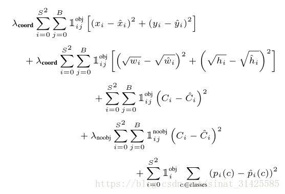
這僅僅是自己學習的一個筆記,如果有地方不妥之處,歡迎大家批評指證,謝謝!
參考資料:
Andrew NG的deeplearning.ai課程