激勵函式簡介 Tensorflow最簡單的三層神經網路及matplotlib視覺化 附激勵函式常見型別
阿新 • • 發佈:2019-02-15
激勵函式:
有人說翻譯成“啟用函式”(activation function)會更好,因為主要作用是分割資料,判斷該“神經”是否被啟用。比如說,當你判斷面前的動物是否是一隻貓的時候,你會從各個部分去判斷。比如眼睛,當你覺得確實像貓的眼睛時,判斷眼睛的神經數值會特別高,如果覺得比較像,則會相對低一點,在神經網路演算法中,可以說,激勵函式就是分割這個神經判斷是與否的準則。 某些資料是可以被線性分割的,但是也有很多資料是不可被線性分割的,因此,激勵函式也是多種多樣的。三層神經網:
以下是一個最簡單的三層神經網路結構,程式碼中都有註釋,輸入層,隱藏層,輸出層。其中,輸入層,輸出層為1個神經元,隱藏層為10個神經元,並且訓練1000次。目的是為了讓x_data資料與y_data資料進行擬合。
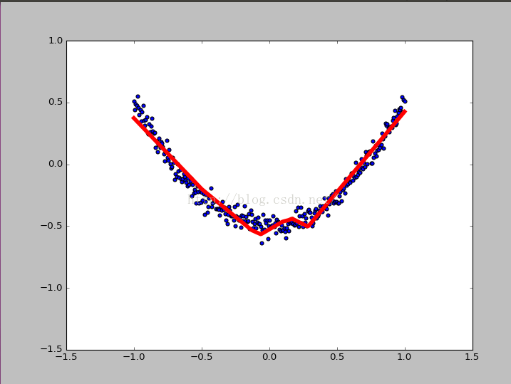
import tensorflow as tf
import numpy as np
import matplotlib.pyplot as plt

def add_layer(inputs,in_size,out_size,activation_function=None): #activation_function=None線性函式
	Weights = tf.Variable(tf.random_normal([in_size,out_size])) #Weight中都是隨機變數
	biases = tf.Variable(tf.zeros([1,out_size])+0.1) #biases推薦初始值不為0
	Wx_plus_b = tf.matmul(inputs,Weights)+biases #inputs*Weight+biases
	if activation_function is None:
		outputs = Wx_plus_b
	else:
		outputs = activation_function(Wx_plus_b)
	return outputs

#建立資料x_data,y_data
x_data = np.linspace(-1,1,300)[:,np.newaxis] #[-1,1]區間,300個單位,np.newaxis增加維度
noise = np.random.normal(0,0.05,x_data.shape) #噪點
y_data = np.square(x_data)-0.5+noise

xs = tf.placeholder(tf.float32,[None,1])
ys = tf.placeholder(tf.float32,[None,1])
#三層神經,輸入層(1個神經元),隱藏層(10神經元),輸出層(1個神經元)
l1 = add_layer(xs,1,10,activation_function=tf.nn.relu) #輸入層
prediction = add_layer(l1,10,1,activation_function=None) #隱藏層

#predition值與y_data差別
loss = tf.reduce_mean(tf.reduce_sum(tf.square(ys-prediction),reduction_indices=[1])) #square()平方,sum()求和,mean()平均值

train_step = tf.train.GradientDescentOptimizer(0.1).minimize(loss) #0.1學習效率,minimize(loss)減小loss誤差

init = tf.initialize_all_variables()
sess = tf.Session()
sess.run(init) #先執行init

#視覺化
fig = plt.figure()
ax = fig.add_subplot(1,1,1)
ax.scatter(x_data,y_data)
plt.ion() #不讓show() block
plt.show()

#訓練1k次
for i in range(1000):
	sess.run(train_step,feed_dict={xs:x_data,ys:y_data})
	if i%50==0:
		try:
			ax.lines.remove(lines[0]) #lines建一個抹除一個
		except Exception:
			pass
		#print(sess.run(loss,feed_dict={xs:x_data,ys:y_data})) #輸出loss值
		#視覺化
		prediction_value = sess.run(prediction,feed_dict={xs:x_data,ys:y_data})
		lines = ax.plot(x_data,prediction_value,'r-',lw=5) #x_data X軸,prediction_value Y軸,'r-'紅線,lw=5線寬5
		plt.pause(0.1) #暫停0.1秒
結果:
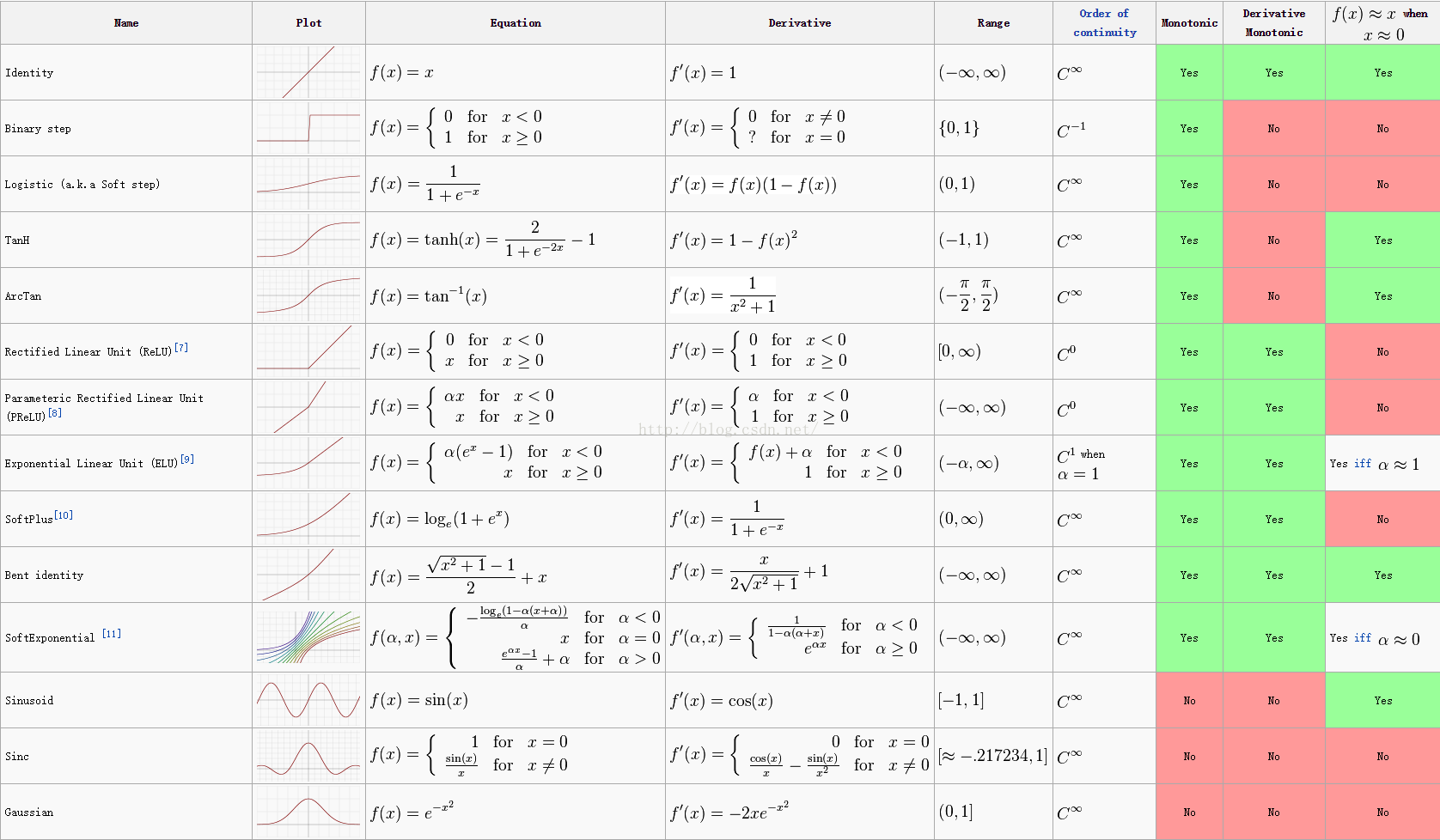
附:常見激勵函式型別: