前言

• 這兩個月真是突如其來的清閒……偶爾分配來個 Bug，但經常就很快搞定了。跟組長討論了一下程式碼結構優化方面的問題，把之前加入的一套業務邏輯做了整體優化，然後又陷入 “閒” 者模式。
• 剩下的大多時間都是在學習學習，熟悉熟悉專案原始碼。現在主要在搞 MTK Camera Hal 層的東西， 真是想吐槽一下，Mtk 的程式碼有很多冗餘的部分，比如各種 CamAdapter，明明程式碼一樣一樣的，非要複製好幾份出來，然後只是在 creatInstance 的時候區分一下……就不捨得提取一些狀態之類的東西出來優化一下……
• 然後編譯的時間經常要很久，sourceInsight 又時不時要同步資訊，各個基線的專案每隔一兩天也得更新一次……趁著這些時間，我就悄悄地繼續投入到翻譯社第二期活動裡去了…..
• 值得一提的是，上期活動貢獻排名前十，騰訊給我發來了一個狗年的公仔 “哈士企”……
• 第二期活動是 “探索AI技術，科技引領未來”，不得不說這正對我胃口，於是多領了幾篇……
• 雖然總共翻譯了十篇文章，但是由於有些文章內容其實比較一般，再一個就是像自然語言處理這方面的內容其實以前並沒有經常看，所以對裡面很多專業的描述表述不清楚，所以很多篇文章都只是通過，沒被專欄採納……

版權相關

翻譯人：StoneDemo，該成員來自雲+社群翻譯社
原文連結：Image Compression with Neural Networks
原文作者：Posted by Nick Johnston and David Minnen

Image Compression with Neural Networks

題目：基於神經網路的影象壓縮技術

Data compression is used nearly everywhere on the internet - the videos you watch online, the images you share, the music you listen to, even the blog you’re reading right now. Compression techniques make sharing the content you want quick and efficient. Without data compression, the time and bandwidth costs for getting the information you need, when you need it, would be exorbitant!

在網際網路之中，資料壓縮技術可以說無處不在 —— 您線上觀看的視訊，分享的圖片，聽到的音樂，甚至是您正在閱讀的這篇部落格。壓縮技術使得您可以快速且高效地分享內容。如果沒有資料壓縮，我們在獲取所需的資訊時，時間與頻寬的開銷會高得難以接受！

In “Full Resolution Image Compression with Recurrent Neural Networks”, we expand on our previous research on data compression using neural networks, exploring whether machine learning can provide better results for image compression like it has for image recognition and text summarization. Furthermore, we are releasing our compression model via TensorFlow so you can experiment with compressing your own images with our network.

在 “基於遞迴神經網路的全解析度影象壓縮 ” 一文中，我們對以往使用神經網路進行資料壓縮的研究進行了拓展，以探索機器學習是否能像在影象識別與文字摘要領域中的表現一樣，提供更好的影象壓縮效果。此外，我們也正通過 TensorFlow 來發布我們的壓縮模​​型，以便您可以嘗試使用我們的網路來壓縮您自己的影象。

We introduce an architecture that uses a new variant of the Gated Recurrent Unit (a type of RNN that allows units to save activations and process sequences) called Residual Gated Recurrent Unit (Residual GRU). Our Residual GRU combines existing GRUs with the residual connections introduced in “Deep Residual Learning for Image Recognition” to achieve significant image quality gains for a given compression rate. Instead of using a DCT to generate a new bit representation like many compression schemes in use today, we train two sets of neural networks - one to create the codes from the image (encoder) and another to create the image from the codes (decoder).

當前我們提出了一種使用殘差門控迴圈單元（RGRU，Residual GRU）的架構，這種單元是門控迴圈單元（GRU，Gated Recurrent Unit，一種允許單元儲存啟用和處理序列的 RNN 型別）的一個新型變體。我們的 RGRU 是將原本的 GRU 與文章 “深度殘差學習影象識別 ” 中引入的殘差連線相結合，以實現在給定的壓縮率下獲得更顯著的影象質量增益。我們訓練了兩組神經網路 —— 一組用於根據影象進行編碼（即作為編碼器），另一組則是從編碼中解析出影象（即解碼器）。而這兩組神經網路則代替了目前影象壓縮技術中主要使用的，採用 DCT（Discrete Cosine Transform，離散餘弦變換） 來生成新的位元表示的壓縮方案。

Our system works by iteratively refining a reconstruction of the original image, with both the encoder and decoder using Residual GRU layers so that additional information can pass from one iteration to the next. Each iteration adds more bits to the encoding, which allows for a higher quality reconstruction. Conceptually, the network operates as follows:

1. The initial residual, R[0], corresponds to the original image I: R[0] = I.
2. Set i=1 for to the first iteration.
3. Iteration[i] takes R[i-1] as input and runs the encoder and binarizer to compress the image into B[i].
4. Iteration[i] runs the decoder on B[i] to generate a reconstructed image P[i].
5. The residual for Iteration[i] is calculated: R[i] = I - P[i].
6. Set i=i+1 and go to Step 3 (up to the desired number of iterations).

我們的系統通過迭代的方式提煉原始影象的重構，同時編碼器和解碼器都使用了 RGRU 層，從而使得附加資訊在多次迭代中傳遞下去。每次迭代都會在編碼中增加更多的位元位數，從而實現更高質量的重構。從概念上來說，該網路的工作流程如下：

1. 初始殘差 R[0] 對應於原始影象 I，即 R[0] = I。
2. 為第一次迭代設定 i = 1。
3. 第 i 次迭代以 R[i-1] 作為輸入，並執行編碼器和二進位制化器將影象壓縮成 B[i]。
4. 第 i 次迭代執行 B[i] 上的解碼器以生成重建的影象 P[i]。
5. 計算第 i 次迭代的殘差：R[i] = I - P[i]。
6. 設定 i = i + 1 並轉到步驟 3（直到達到了所需的迭代次數為止）。

The residual image represents how different the current version of the compressed image is from the original. This image is then given as input to the network with the goal of removing the compression errors from the next version of the compressed image. The compressed image is now represented by the concatenation of B[1] through B[N]. For larger values of N, the decoder gets more information on how to reduce the errors and generate a higher quality reconstruction of the original image.

殘差影象展示了當前版本的壓縮影象與原始影象的差異。而該影象隨後則作為輸入提供給神經網路，其目的是剔除下一版本的壓縮影象中的壓縮錯誤。現在壓縮的影象則是由 B[1] 至 B[N] 的連線表示。N 值越大，解碼器就能獲得更多有助於減少錯誤，同時又可以生成更高質量的原始影象的重構的資訊。

To understand how this works, consider the following example of the first two iterations of the image compression network, shown in the figures below. We start with an image of a lighthouse. On the first pass through the network, the original image is given as an input (R[0] = I). P[1] is the reconstructed image. The difference between the original image and encoded image is the residual, R[1], which represents the error in the compression.

為了理解該演算法是如何運作的，請考慮如下圖所示的，影象壓縮網路前兩次迭代的示例。我們以一座燈塔的影象作為原始資料。當它第一次通過網路時，原始影象作為輸入進入（R[0] = I）。P[1] 是重建的影象。原始影象和編碼影象之間的差異即是殘差 R[1]，它表示了壓縮中出現的誤差。

（左圖：原始影象，I = R[0]。中圖：重建的影象，P[1]。右：表示由壓縮引入的錯誤的殘差 R[1]。）

On the second pass through the network, R[1] is given as the network’s input (see figure below). A higher quality image P[2] is then created. So how does the system recreate such a good image (P[2], center panel below) from the residual R[1]? Because the model uses recurrent nodes with memory, the network saves information from each iteration that it can use in the next one. It learned something about the original image in Iteration[1] that is used along with R[1] to generate a better P[2] from B[2]. Lastly, a new residual, R[2] (right), is generated by subtracting P[2] from the original image. This time the residual is smaller since there are fewer differences between the reconstructed image, and what we started with.

在第二次通過網路時，R[1] 則作為網路的輸入（如下圖）。然後更高質量的影象 P[2] 就生成了。那麼問題來了，系統是如何根據輸入的殘差 R[1] 重新創建出這樣一個更好的影象（P[2]，下圖中部）的呢？這是由於模型使用了帶有記憶功能的迴圈節點，因此網路會儲存每次迭代中可用於下一次迭代的資訊。它在第一次迭代中學習到了關於原始影象的一些東西，這些東西同 R[1] 一起用於從 B[2] 中生成更好的 P[2]。最後，通過從原始影象中減去 P[2] 就產生了新的殘差 R[2]（右）。由於本次我們重建得到的影象和原始影象之間的差異較小，因此殘差也較小。

（第二遍通過網路。左圖：R[1] 作為輸入。中圖：更高質量的重建，P[2]。右圖：通過從原始影象中減去 P[2] 生成更小的殘差 R[2]。）

At each further iteration, the network gains more information about the errors introduced by compression (which is captured by the residual image). If it can use that information to predict the residuals even a little bit, the result is a better reconstruction. Our models are able to make use of the extra bits up to a point. We see diminishing returns, and at some point the representational power of the network is exhausted.

在之後的每次迭代中，網路將獲得更多由於壓縮而引入的誤差的資訊（通過殘差影象捕獲到的資訊）。如果我們可以用這些資訊來預測殘差，那麼就能得到更優重建結果。我們的模型能夠在一定程度上利用多餘的部分資訊。我們可以看到收益是遞減的，並且在某個時候，網路的所表現出來的能力就會被用盡。

To demonstrate file size and quality differences, we can take a photo of Vash, a Japanese Chin, and generate two compressed images, one JPEG and one Residual GRU. Both images target a perceptual similarity of 0.9 MS-SSIM, a perceptual quality metric that reaches 1.0 for identical images. The image generated by our learned model results in an file 25% smaller than JPEG.

為了演示檔案大小和質量之間的差異，我們可以拍攝一張日本狆 Vash 的照片，並生成兩種壓縮影象，一個 JPEG 和一個 RGRU。兩幅影象都以 0.9 MS-SSIM 的感知相似度為目標，如果是兩張完全相同的影象，它們之間的感知相似度就是 1.0。我們的學習模型在同樣質量的情況下，生成了比 JPEG 小 25％ 的最終影象。

（左圖：1.0 MS-SSIM 的原始影象（1419 KB PNG）。中圖：0.9 MS-SSIM 的 JPEG（33 KB）。右圖：0.9 MS-SSIM 的 RGRU（24 KB）。相比之下，影象資料量要小25％）

Taking a look around his nose and mouth, we see that our method doesn’t have the magenta blocks and noise in the middle of the image as seen in JPEG. This is due to the blocking artifacts produced by JPEG, whereas our compression network works on the entire image at once. However, there’s a tradeoff – in our model the details of the whiskers and texture are lost, but the system shows great promise in reducing artifacts.

觀察它的鼻子和嘴巴，我們可以看到，我們的方法沒有造成在 JPEG 影象中看到的中間部分的洋紅色塊和噪音。這是由於 JPEG 壓縮的方塊效應而產生的，而此處我們的壓縮網路對整個影象同時處理。然而，這是經過了權衡的 —— 在我們的模型中，晶須和紋理的細節丟失了，但是它在減少方塊效應方面展現出了強大能力。

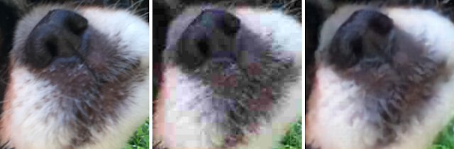
（左圖：原始影象。中圖： JPEG。右圖：RGRU。）

While today’s commonly used codecs perform well, our work shows that using neural networks to compress images results in a compression scheme with higher quality and smaller file sizes. To learn more about the details of our research and a comparison of other recurrent architectures, check out our paper. Our future work will focus on even better compression quality and faster models, so stay tuned!

雖然今天我們常用的編解碼器依舊錶現良好，但我們的工作已經表明，使用神經網路來壓縮影象可以生成質量更高且資料量更小的壓縮方案。如果想了解更多關於我們的研究的細節，以及與其他迴圈架構的比較，請檢視我們的論文。在未來的研究中，我們將著重於獲得更好的壓縮質量以及設計更高效的模型，敬請期待！