import pandas as pd
import numpy as np
import warnings
from matplotlib import pyplot
#from pandas import read_csv, set_option
from pandas import Series, datetime
from pandas.tools.plotting import scatter_matrix, autocorrelation_plot
from sklearn.preprocessing import StandardScaler
from sklearn.model_selection import train_test_split, KFold, cross_val_score, GridSearchCV, TimeSeriesSplit
from sklearn.metrics import classification_report, confusion_matrix, accuracy_score, mean_squared_error
from sklearn.pipeline import Pipeline
from sklearn.linear_model import LogisticRegression
from sklearn.tree import DecisionTreeClassifier
from sklearn.neighbors import KNeighborsClassifier
from sklearn.discriminant_analysis import LinearDiscriminantAnalysis
from sklearn.naive_bayes import GaussianNB
from sklearn.svm import SVC
from sklearn.ensemble import AdaBoostClassifier, GradientBoostingClassifier, RandomForestClassifier, ExtraTreesClassifier
from sklearn.metrics import roc_curve, auc
import matplotlib.pyplot as plt
import random
from statsmodels.graphics.tsaplots import plot_acf, plot_pacf
from statsmodels.tsa.arima_model import ARIMA
from xgboost import XGBClassifier
import seaborn as sns

每次引入資料，都應該檢查其規模大小，資料型別，對資料有一個大致瞭解

sentence_file = "combined_stock_data.csv"
sentence_df = pd.read_csv(sentence_file, parse_dates=[1])#parse_dates is used to 指定時間序列

print(sentence_df.shape)
print(sentence_df.dtypes)
print(sentence_df)

stock_prices = "DJIA_table.csv"
stock_data = pd.read_csv(stock_prices,parse_dates=[0])
stock_data.head()

#by checking the head or tail we can have an overview of the data
 

#你會發現Volumn是int型，為了保持所有資料型別的一致性
#應該把資料轉換為float
print(stock_data.shape)
print(stock_data.dtypes)

merged_dataframe = sentence_df[['Date','Label','Subjectivity','Objectivity','Positive', 'Negative', 'Neutral']].merge(stock_data, how='inner', on='Date', left_index=True)
print(merged_dataframe.shape)
merged_dataframe.head()
 

merged_dataframe['Volume']=merged_dataframe['Volume'].astype(float)

print(merged_dataframe.dtypes)
#recheck

cols=list(merged_dataframe)
print(cols)
cols.append(cols.pop(cols.index('Label')))
merged_dataframe=merged_dataframe.ix[:,cols]
merged_dataframe.head()

del merged_dataframe['Volume']

merged_dataframe.head()

#w我們做到這裡，是data preparation 
#包括資料的整合，資料型別的統一，資料順序的微調


#接下來進行資料質量的檢測
#看缺失值和極端值的影響

#describe()  用來巨集觀觀察資料的質量

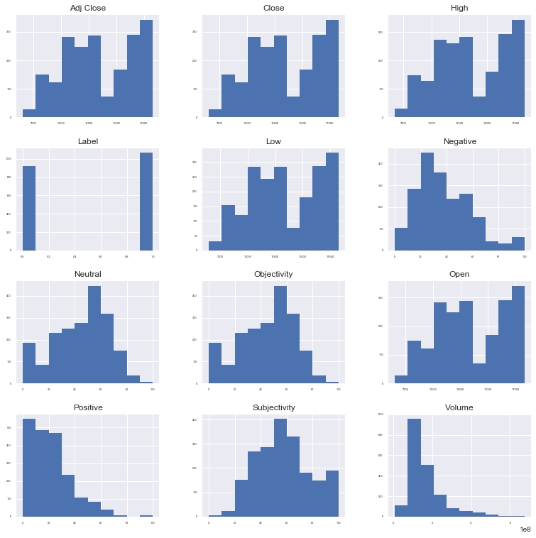
print(merged_dataframe.describe())

#對所有資料的畫圖，看分佈
#x軸是列值，y軸是頻數
sns.set()
merged_dataframe.hist(sharex = False, sharey = False, xlabelsize = 4, ylabelsize = 4, figsize=(13, 13))
pyplot.show()

#如果資料分佈不均勻的話，要進行進一部分變換，使得資料的分佈更加均勻

pyplot.scatter(merged_dataframe['Subjectivity'],merged_dataframe['Label'])
pyplot.xlabel('Subjectivity')
pyplot.ylabel('Stock Price Up or Down 0: Down, 1: Up')
pyplot.show()
pyplot.scatter(merged_dataframe['Objectivity'], merged_dataframe['Label'])
pyplot.xlabel('Objectivity')
pyplot.ylabel('Stock Price Up or Down 0: Down, 1: Up')
pyplot.show()

merged_dataframe['Subjectivity'].plot('hist')
pyplot.xlabel('Subjectivity')
pyplot.ylabel('Frequency')
pyplot.show()

merged_dataframe['Objectivity'].plot('hist')
pyplot.xlabel('Objectivity')
pyplot.ylabel('Frequency')
pyplot.show()

print("Size of the Labels column")
print(merged_dataframe.groupby('Label').size())

#如何知道各列之間的關係呢？
#畫一個Correlation Map
# plot a heat map and a scatter matrix
#一些機器學習演算法要求變數之間不能有強關聯關係，這種情況下就需要降維
colormap = pyplot.cm.afmhot
pyplot.figure(figsize=(16,12))
pyplot.title('Pearson correlation of continuous features', y=1.05, size=15)
sns.heatmap(merged_dataframe.corr(),linewidths=0.1,vmax=1.0, square=True, 
            cmap=colormap, linecolor='white', annot=True)
pyplot.show()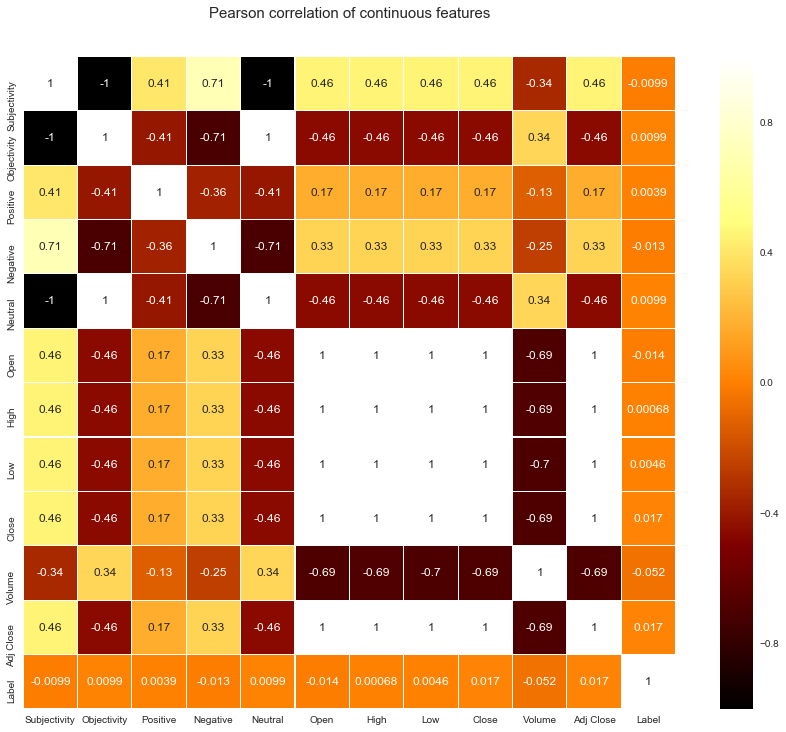

md_copy.index = md_copy.index.sort_values() ##important!

merged_dataframe=md_copy
print(merged_dataframe.dtypes)
print(merged_dataframe.count())
# Change the NaN values to the mean value of that column
nan_list = ['Subjectivity', 'Objectivity', 'Positive', 'Negative', 'Neutral']
for col in nan_list:
    merged_dataframe[col] = merged_dataframe[col].fillna(merged_dataframe[col].mean())

# Recheck the count
print(merged_dataframe.count())
# Separate the dataframe for input(X) and output variables(y)
X = merged_dataframe.loc[:,'Subjectivity':'Adj Close']
y = merged_dataframe.loc[:,'Label']
# Set the validation size, i.e the test set to 20%
validation_size = 0.20
# Split the dataset to test and train sets
# Split the initial 70% of the data as training set and the remaining 30% data as the testing set
train_size = int(len(X.index) * 0.7)
print(len(y))
print(train_size)
X_train, X_test = X.loc[0:train_size, :], X.loc[train_size: len(X.index), :]
y_train, y_test = y[0:train_size+1], y.loc[train_size: len(X.index)]
print('Observations: %d' % (len(X.index)))
print('X Training Observations: %d' % (len(X_train.index)))
print('X Testing Observations: %d' % (len(X_test.index)))
print('y Training Observations: %d' % (len(y_train)))
print('y Testing Observations: %d' % (len(y_test)))
pyplot.plot(X_train['Objectivity'])
pyplot.plot([None for i in X_train['Objectivity']] + [x for x in X_test['Objectivity']])
pyplot.show()
num_folds = 10
scoring = 'accuracy'
# Append the models to the models list
models = []
models.append(('LR' , LogisticRegression()))
models.append(('LDA' , LinearDiscriminantAnalysis()))
models.append(('KNN' , KNeighborsClassifier()))
models.append(('CART' , DecisionTreeClassifier()))
models.append(('NB' , GaussianNB()))
models.append(('SVM' , SVC()))
models.append(('RF' , RandomForestClassifier(n_estimators=50)))
models.append(('XGBoost', XGBClassifier()))

Date            datetime64[ns]
Subjectivity           float64
Objectivity            float64
Positive               float64
Negative               float64
Neutral                float64
Open                   float64
High                   float64
Low                    float64
Close                  float64
Adj Close              float64
Label                    int64
dtype: object
Date            1989
Subjectivity    1986
Objectivity     1986
Positive        1986
Negative        1986
Neutral         1986
Open            1989
High            1989
Low             1989
Close           1989
Adj Close       1989
Label           1989
dtype: int64
Date            1989
Subjectivity    1989
Objectivity     1989
Positive        1989
Negative        1989
Neutral         1989
Open            1989
High            1989
Low             1989
Close           1989
Adj Close       1989
Label           1989
dtype: int64
1989
1392
Observations: 1989
X Training Observations: 1393
X Testing Observations: 597
y Training Observations: 1393
y Testing Observations: 597

results =[]
for name,model in models:
    clf = model
    clf.fit(X_train,y_train)
    y_pred = clf.predict(X_test)
    accu_score = accuracy_score(y_test,y_pred)
    print(name+ ":"+str(accu_score))
    
#XGboost 與 LDA最高
#但是LDA是可信的嗎？？

LR:0.9715242881072027

LDA:0.9413735343383585
KNN:0.609715242881072
CART:0.5209380234505863
NB:0.49748743718592964
SVM:0.5309882747068677
RF:0.5527638190954773
XGBoost:0.5862646566164154

scaler = StandardScaler().fit(X_train)
rescaledX = scaler.transform(X_train)
model_lda = LinearDiscriminantAnalysis()
model_lda.fit(rescaledX,y_train)

#estimate accuracy on validation dataset

rescaledValidationX = scaler.transform(X_test)

predictions = model_lda.predict(rescaledValidationX)
print("accuracy score:")
print(accuracy_score(y_test,predictions))
print("confusion matrix")
print(confusion_matrix(y_test,predictions))

print("classification report")
print(classification_report(y_test,predictions))#很有用哦，返回準確率，召回率

accuracy score:
0.9413735343383585
confusion matrix
[[252  28]
 [  7 310]]
classification report
             precision    recall  f1-score   support

          0       0.97      0.90      0.94       280
          1       0.92      0.98      0.95       317

avg / total       0.94      0.94      0.94       597

#當data都在不同範圍的時候，最好用feature scaling歸一化
scaler = StandardScaler().fit(X_train)
rescaledX = scaler.transform(X_train)

model_xgb = XGBClassifier()
model_xgb.fit(rescaledX,y_train)

rescaledValidationX = scaler.transform(X_test)
predictions = model_xgb.predict(rescaledValidationX)

print("accuracy score:")
print(accuracy_score(y_test, predictions))
print("confusion matrix: ")
print(confusion_matrix(y_test, predictions))
print("classification report: ")
print(classification_report(y_test, predictions))

#接下來畫ROC/AUC來判別LDA的結果是否可信
#generating the roc curve
y_pred_proba = model_lda.predict_proba(X_test)[:,1]
#第 i 行 第 j 列上的數值是模型預測 第 i 個預測樣本為某個標籤的概率，並且每一行的概率和為1。

fpr,tpr,thresholds = roc_curve(y_test,y_pred_proba)
roc_auc = auc(fpr,tpr)

#plot ROC curve
print("roc auc is :" +str(roc_auc))

pyplot.plot([0,1],[0,1],'k--')
pyplot.plot(fpr,tpr)
pyplot.xlabel('False Positive Rate')
pyplot.ylabel('True Positive Rate')
pyplot.title('Roc Curve')
pyplot.show()

kfold_val = KFold(n_splits = num_folds,random_state = 42)
auc_score = cross_val_score(model_lda,X_test,y_test,cv=kfold_val,scoring = 'roc_auc')
print("AUC using cross val: "+str(auc_score))
mean_auc = np.mean(auc_score)
print("Mean AUC score is: "+str(mean_auc))

#Scaling Random Forests
model_rf = RandomForestClassifier(n_estimators=1000)
model_rf.fit(rescaledX,y_train)

#estimate accuracy on validation dataset
rescaledValidationX = scaler.transform(X_test)
predictions = model_rf.predict(rescaledValidationX)


print("accuracy score:")
print(accuracy_score(y_test, predictions))
print("confusion matrix: ")
print(confusion_matrix(y_test, predictions))
print("classification report: ")
print(classification_report(y_test, predictions))

accuracy score:
0.5644891122278057
confusion matrix: 
[[102 178]
 [ 82 235]]
classification report: 
             precision    recall  f1-score   support

          0       0.55      0.36      0.44       280
          1       0.57      0.74      0.64       317

avg / total       0.56      0.56      0.55       597

#fine tuning XGBoost
#主要用來調參的是 n_estimators 和 max_depth

#n_estimator:XGBoost is an additive model, multiple models are created on different samples of data and the model learns after training of different samples. How many samples are the optimum best for the XGBoost to train from is usually unknown and the best way to find out is to check by training on different set of estimators.'

#model selection 
from sklearn.model_selection import GridSearchCV
from sklearn.model_selection import StratifiedKFold
from sklearn.preprocessing import LabelEncoder
#ignore warnings
import warnings
warnings.filterwarnings("ignore")



n_estimators = [150,200,250,300,450,500,550,600,800,1000]
max_depth=[i for i in range(1,12)]
print(max_depth)

#initialize best depth,best score,best estimator


max_score = 0
best_depth = 0
best_estimator = 0



for n in n_estimators:
    for md in max_depth:
        model = XGBClassifier(n_estimators = n,max_depth = md)
        model.fit(X_train,y_train)
        y_pred = model.predict(X_test)
        score = accuracy_score(y_test,y_pred)
        if score>max_score:
            max_score = score
            best_depth = md
            best_estimator = n
        #print("score is: "+str(score)+"at depth of "+str(md)+"and estimator"+str(n))

print("Best score is " + str(max_score) + " at depth of " + str(best_depth) + " and estimator of " + str(best_estimator))

#結果顯示depth 3 和 estimator 500結果最佳，準確率上升到0.616

#這個過程有點久，慢慢等

#？？準確率居然還下降了
imp_features_df = merged_dataframe[['Low', "Neutral", 'Close', 'Objectivity']]
Xi_train, Xi_test = imp_features_df.loc[0:train_size, :], imp_features_df.loc[train_size: len(X.index), :]
clf = XGBClassifier(n_estimators=500, max_depth=3)
clf.fit(Xi_train, y_train)
yi_pred = clf.predict(Xi_test)
score = accuracy_score(y_test, yi_pred)
print("Score is "+ str(score))

from sklearn.decomposition import PCA

pca = PCA(n_components=3)
pca.fit(X)
transformed = pca.transform(X)

print(transformed.shape)
print(type(transformed))

pca_df = pd.DataFrame(transformed)

X_train_pca,X_test_pca = pca_df.loc[0:train_size,:],pca_df.loc[train_size:len(X.index),:]

clf = XGBClassifier(n_estimators = 500,max_depth = 3)

clf.fit(X_train_pca,y_train)

y_pred_pca =clf.predict(X_test_pca)

score = accuracy_score(y_test,y_pred_pca)

print("Score is "+str(score))

#但結果不一定可信，還是得看confusion_matrix 以及classification_report


pca_matrix = confusion_matrix(y_test,y_pred_pca)
pca_report = classification_report(y_test,y_pred_pca)
print("Confusion Matrix: \n" + str(pca_matrix))
print("Classification report: \n" + str(pca_report))

Score is 0.9547738693467337
Confusion Matrix: 
[[266  14]
 [ 13 304]]
Classification report: 
             precision    recall  f1-score   support

          0       0.95      0.95      0.95       280
          1       0.96      0.96      0.96       317

avg / total       0.95      0.95      0.95       597

y_pred_proba_pca = clf.predict_proba(X_test_pca)[:,1]
fpr,tpr,thresholds = roc_curve(y_test,y_pred_proba_pca)
roc_auc = auc(fpr,tpr)
print("AUC score is "+str(roc_auc))

print("roc auc is : "+str(roc_auc))
pyplot.plot([0, 1], [0, 1], 'k--')
pyplot.plot(fpr, tpr)
pyplot.xlabel('False Positive Rate')
pyplot.ylabel('True Positive Rate')
pyplot.title('ROC Curve')
pyplot.show()

AUC score is 0.9857875168995043
roc auc is : 0.9857875168995043

說明結果可信度還是蠻高的。