
神經網路 手寫識別例子 matlab實現
阿新 • • 發佈:2019-02-20
Model representation
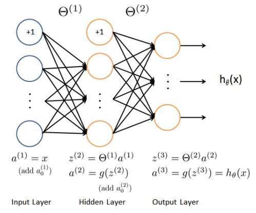
作為例子模型,神經網路有三層,一個輸入層,一個隱藏層和一個輸出層。
在手寫數字識別中,輸入是20*20的圖片畫素值,因此輸入層除偏差單元1外,有400個單元。
第二層有25個單元;輸出層有10單元,對應識別的數字(類),0用10來表示。
訓練集依舊用X,y來表示。
中間引數為Theta1和Theta2。
Load data and set parameters
.mat格式的資料檔案,直接儲存了X,y。
fileName = 'xxx.mat';
load(fileName, 'X', 'y');
m = size(X, 1);
input_layer_size = 400 Visualize data
隨機選擇100個數據點,視覺化。
randperm(n),可以把隨機打亂一個n長度的數字序列。
sel = randperm(m);
sel = sel(1:100);

displayData(X(sel, :));
displayData函式
function [h, display_array] = displayData(X, example_width)
%DISPLAYDATA Display 2D data in a nice grid
% [h, display_array] = DISPLAYDATA(X, example_width) displays 2D data
% stored in X in a nice grid. It returns the figure handle h and the
% displayed array if requested. Train parameters
Random initialize Theta
% 隨機初始化theta
initial_Theta1 = randInitializeWeights(input_layer_size, hidden_layer_size);
initial_Theta2 = randInitializeWeights(hidden_layer_size, num_labels);
% 將引數合併,便於傳參
initial_nn_params = [initial_Theta1(:) ; initial_Theta2(:)];
randInitializeWeights函式
function W = randInitializeWeights(L_in, L_out)
    W = zeros(L_out, 1 + L_in);

    epsilon_init = sqrt(6) / sqrt(L_in + L_out);
    W = rand(L_out, 1 + L_in) * 2 * epsilon_init - epsilon_init;
end
Cost Function
首先Feedforward算出
接著用backpropagation計算Theta_grad的值,其過程如下:
對每一個樣例t=1:m
- 對在輸出層的每個輸出單元k(例子,第3層),
δ(3)k=(a(3)k−yk) ,其中yk∈{0,1} ,為1資料類k,反之不屬於。 - 對隱藏層
l=2 ,δ(2)=(θ(2))Tδ(3).∗g′(z(2)) - 只去掉輸入層後一層的
δ 的首行值,接著累加grad=grad+δ(l+1)(a(l))T grad=1mgrad - 正規化
costFunction函式
function [J grad] = CostFunction(nn_params, ...
                                   input_layer_size, ...
                                   hidden_layer_size, ...
                                   num_labels, ...
                                   X, y, lambda)

    m = size(X, 1);

    Theta1 = reshape(nn_params(1:hidden_layer_size * (input_layer_size + 1)), ...
                     hidden_layer_size, (input_layer_size + 1));

    Theta2 = reshape(nn_params((1 + (hidden_layer_size * (input_layer_size + 1))):end), ...
                     num_labels, (hidden_layer_size + 1));

    J = 0;
    Theta1_grad = zeros(size(Theta1));
    Theta2_grad = zeros(size(Theta2));

% Feedforward
    a1 = [ones(m, 1) X];
    z2 = a1 * Theta1';
    a2 = [ones(m, 1) sigmoid( z2 )];
    z3 = a2 * Theta2';
    a3 = sigmoid( z3 );
    hx = a3;

    for i = 1 : m
        y_vec = zeros(1, num_labels);
        y_vec(y(i)) = 1;
        J = J + sum( -y_vec .* log(hx(i, :)) - (1 - y_vec) .* log(1 - hx(i, :)) );
    end
    J = J / m;
    J = J + lambda/(2*m) * (sum(sum(Theta1(:,2:end).^2))+sum(sum(Theta2(:,2:end).^2)));

% backpropagation
    for i = 1 : m
        y_vec = zeros(1, num_labels);
        y_vec(y(i)) = 1;
        delta3 = a3(i, :) - y_vec; %1 10
        delta2 = delta3 * Theta2 .* [0 sigmoidGradient(z2(i, :))]; %1 26
        delta2 = delta2(2 : end); %1 25
        Theta2_grad = Theta2_grad + delta3' * a2(i, :);
        Theta1_grad = Theta1_grad + delta2' * a1(i, :);
    end
    Theta2_grad = Theta2_grad / m;
    Theta1_grad = Theta1_grad / m;

% regularization
    Theta1(:, 1) = 0;
    Theta1_grad = Theta1_grad + lambda / m * Theta1;
    Theta2(:, 1) = 0;
    Theta2_grad = Theta2_grad + lambda / m * Theta2;

    grad = [Theta1_grad(:) ; Theta2_grad(:)];

end
sigmoid函式
function g = sigmoid(z)
    g = 1.0 ./ (1.0 + exp(-z));
end
sigmoid求導函式
function g = sigmoidGradient(z)
    g = sigmoid(z);
    g = g .* ( 1 - g );
end
Train
呼叫fmincg來訓練,這個函式是octave裡的函式。
使用fminunc和fminsearch都會宕機,原因應該是資料量太大了。
options = optimset('MaxIter', 50);
lambda = 1;

f = @(p) CostFunction(p, ...
                        input_layer_size, ...
                        hidden_layer_size, ...
                        num_labels, X, y, lambda);

[nn_params, cost] = fmincg(f, initial_nn_params, options);

Theta1 = reshape(nn_params(1:hidden_layer_size * (input_layer_size + 1)), ...
                 hidden_layer_size, (input_layer_size + 1));

Theta2 = reshape(nn_params((1 + (hidden_layer_size * (input_layer_size + 1))):end), ...
                 num_labels, (hidden_layer_size + 1));
fmincg函式
function [X, fX, i] = fmincg(f, X, options, P1, P2, P3, P4, P5)
% Minimize a continuous differentialble multivariate function. Starting point
% is given by "X" (D by 1), and the function named in the string "f", must
% return a function value and a vector of partial derivatives. The Polack-
% Ribiere flavour of conjugate gradients is used to compute search directions,
% and a line search using quadratic and cubic polynomial approximations and the
% Wolfe-Powell stopping criteria is used together with the slope ratio method
% for guessing initial step sizes. Additionally a bunch of checks are made to
% make sure that exploration is taking place and that extrapolation will not
% be unboundedly large. The "length" gives the length of the run: if it is
% positive, it gives the maximum number of line searches, if negative its
% absolute gives the maximum allowed number of function evaluations. You can
% (optionally) give "length" a second component, which will indicate the
% reduction in function value to be expected in the first line-search (defaults
% to 1.0). The function returns when either its length is up, or if no further
% progress can be made (ie, we are at a minimum, or so close that due to
% numerical problems, we cannot get any closer). If the function terminates
% within a few iterations, it could be an indication that the function value
% and derivatives are not consistent (ie, there may be a bug in the
% implementation of your "f" function). The function returns the found
% solution "X", a vector of function values "fX" indicating the progress made
% and "i" the number of iterations (line searches or function evaluations,
% depending on the sign of "length") used.
%
% Usage: [X, fX, i] = fmincg(f, X, options, P1, P2, P3, P4, P5)
%
% See also: checkgrad
%
% Copyright (C) 2001 and 2002 by Carl Edward Rasmussen. Date 2002-02-13
%
%
% (C) Copyright 1999, 2000 & 2001, Carl Edward Rasmussen
%
% Permission is granted for anyone to copy, use, or modify these
% programs and accompanying documents for purposes of research or
% education, provided this copyright notice is retained, and note is
% made of any changes that have been made.
%
% These programs and documents are distributed without any warranty,
% express or implied. As the programs were written for research
% purposes only, they have not been tested to the degree that would be
% advisable in any important application. All use of these programs is
% entirely at the user's own risk.
%
% [ml-class] Changes Made:
% 1) Function name and argument specifications
% 2) Output display
%
% Read options
if exist('options', 'var') && ~isempty(options) && isfield(options, 'MaxIter')
length = options.MaxIter;
else
length = 100;
end
RHO = 0.01; % a bunch of constants for line searches
SIG = 0.5; % RHO and SIG are the constants in the Wolfe-Powell conditions
INT = 0.1; % don't reevaluate within 0.1 of the limit of the current bracket
EXT = 3.0; % extrapolate maximum 3 times the current bracket
MAX = 20; % max 20 function evaluations per line search
RATIO = 100; % maximum allowed slope ratio
argstr = ['feval(f, X']; % compose string used to call function
for i = 1:(nargin - 3)
argstr = [argstr, ',P', int2str(i)];
end
argstr = [argstr, ')'];
if max(size(length)) == 2, red=length(2); length=length(1); else red=1; end
S=['Iteration '];
i = 0; % zero the run length counter
ls_failed = 0; % no previous line search has failed
fX = [];
[f1 df1] = eval(argstr); % get function value and gradient
i = i + (length<0); % count epochs?!
s = -df1; % search direction is steepest
d1 = -s'*s; % this is the slope
z1 = red/(1-d1); % initial step is red/(|s|+1)
while i < abs(length) % while not finished
i = i + (length>0); % count iterations?!
X0 = X; f0 = f1; df0 = df1; % make a copy of current values
X = X + z1*s; % begin line search
[f2 df2] = eval(argstr);
i = i + (length<0); % count epochs?!
d2 = df2'*s;
f3 = f1; d3 = d1; z3 = -z1; % initialize point 3 equal to point 1
if length>0, M = MAX; else M = min(MAX, -length-i); end
success = 0; limit = -1; % initialize quanteties
while 1
while ((f2 > f1+z1*RHO*d1) || (d2 > -SIG*d1)) && (M > 0)
limit = z1; % tighten the bracket
if f2 > f1
z2 = z3 - (0.5*d3*z3*z3)/(d3*z3+f2-f3); % quadratic fit
else
A = 6*(f2-f3)/z3+3*(d2+d3); % cubic fit
B = 3*(f3-f2)-z3*(d3+2*d2);
z2 = (sqrt(B*B-A*d2*z3*z3)-B)/A; % numerical error possible - ok!
end
if isnan(z2) || isinf(z2)
z2 = z3/2; % if we had a numerical problem then bisect
end
z2 = max(min(z2, INT*z3),(1-INT)*z3); % don't accept too close to limits
z1 = z1 + z2; % update the step
X = X + z2*s;
[f2 df2] = eval(argstr);
M = M - 1; i = i + (length<0); % count epochs?!
d2 = df2'*s;
z3 = z3-z2; % z3 is now relative to the location of z2
end
if f2 > f1+z1*RHO*d1 || d2 > -SIG*d1
break; % this is a failure
elseif d2 > SIG*d1
success = 1; break; % success
elseif M == 0
break; % failure
end
A = 6*(f2-f3)/z3+3*(d2+d3); % make cubic extrapolation
B = 3*(f3-f2)-z3*(d3+2*d2);
z2 = -d2*z3*z3/(B+sqrt(B*B-A*d2*z3*z3)); % num. error possible - ok!
if ~