
一個植物轉錄組專案的實戰
轉錄組
轉錄組測序的研究物件為特定細胞在某一功能狀態下所能轉錄出來的所有 RNA 的總和,包括 mRNA 和非編碼 RNA 。通過轉錄組測序,能夠全面獲得物種特定組織或器官的轉錄本資訊,從而進行轉錄本結構研究、變異研究、基因表達水平研究以及全新轉錄本發現等研究。
其中,基因表達水平的探究是轉錄組領域最熱門的方向,利用轉錄組資料來識別轉錄本和表達定量,是轉錄組資料的核心作用。由於這個作用,他可以不依賴其他組學資訊,單獨成為一個產品專案RNA-seq測序。所以很多時候轉錄組測序會與RNA-seq混為一談。
現在RNA-seq資料使用廣泛,但是沒有一套流程可以解決所有的問題。比較值得關注的RNA-seq分析中的重要的步驟包括:實驗設計,質控,read比對,表達定量,視覺化,差異表達,識別可變剪下,功能註釋,融合基因檢測,eQTL定位
值得一提的是,這個教程也寫的非常贊:https://github.com/twbattaglia/RNAseq-workflow
流程介紹
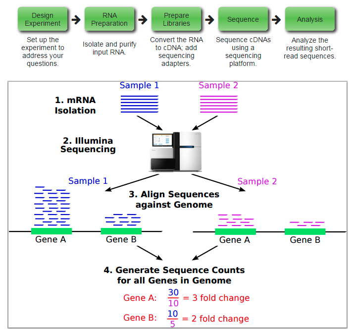
來自於R處理mRNA-seq資料
來自於2010發表在Genome Biology的From RNA-seq reads to differential expression results文章配圖
資料來源文章
資料來自於發表在Nature commmunication 上的一篇文章 “Temporal dynamics of gene expression and histone marks at the Arabidopsis shoot meristem during flowerin”。原文用RNA-Seq的方式研究在開花階段,芽分生組織在不同時期的基因表達變化。
原文的流程是: TopHat -> SummarizeOverlaps -> Deseq2 -> AmiGO其中比對的參考基因組為TAIR10 ver.24 ,並且遮蔽了ribosomal RNA regions (2:3471–9557; 3:14,197,350–14,203,988)。
Deseq2只計算至少在一個時間段的FPKM的count > 1 的基因。
資料存放在http://www.ebi.ac.uk/arrayexpress/, ID為E-MTAB-5130。
實驗設計: 4個時間段(0,1,2,3),分別有4個生物學重複,一共有16個樣品。
資料下載
conda install -c bioconda salmon
wget http://www.ebi.ac.uk/arrayexpress/files/E-MTAB-5130/E-MTAB-5130.sdrf.txt
head -n1 E-MTAB-5130.sdrf.txt | tr '\t' '\n' | nl | grep URI
tail -n +2 E-MTAB-5130.sdrf.txt | cut -f 33 | xargs -i wget {}
nohup wget ftp://ftp.ensemblgenomes.org/pub/plants/release-28/fasta/arabidopsis_thaliana/cdna/Arabidopsis_thaliana.TAIR10.28.cdna.all.fa.gz &
nohup wget ftp://ftp.ensemblgenomes.org/pub/plants/release-28/fasta/arabidopsis_thaliana/dna/Arabidopsis_thaliana.TAIR10.28.dna.genome.fa.gz &
nohup wget ftp://ftp.ensemblgenomes.org/pub/plants/release-28/gff3/arabidopsis_thaliana/Arabidopsis_thaliana.TAIR10.28.gff3.gz &
nohup wget ftp://ftp.ensemblgenomes.org/pub/plants/release-28/gtf/arabidopsis_thaliana/Arabidopsis_thaliana.TAIR10.28.gtf.gz &salmon 流程
軟體介紹:ome of the upstream quantification methods(Salmon,Sailfish,kallisto)are substantially faster and require less memory and disk usage compared to alignment-based methods that require creation and storage of BAM files
軟體官網:https://combine-lab.github.io/salmon/
先用用Salmon建立索引:
- salmon index -t Arabidopsis_thaliana.TAIR10.28.cdna.all.fa.gz -i athal_index
建立索引耗時53秒,生成的索引資料夾如下:
[[email protected] salmon]$ ls -lh
total 19M
-rw-rw-r-- 1 jianmingzeng jianmingzeng  19M Oct 17 11:18 Arabidopsis_thaliana.TAIR10.28.cdna.all.fa.gz
drwxrwxr-x 2 jianmingzeng jianmingzeng 4.0K Oct 17 11:54 athal_index
-rw-rw-r-- 1 jianmingzeng jianmingzeng  142 Oct 17 11:20 wget_cdna.sh
[[email protected] salmon]$ ls -lh  athal_index/
total 1.1G
-rw-rw-r-- 1 jianmingzeng jianmingzeng 751M Oct 17 11:54 hash.bin
-rw-rw-r-- 1 jianmingzeng jianmingzeng  357 Oct 17 11:54 header.json
-rw-rw-r-- 1 jianmingzeng jianmingzeng  115 Oct 17 11:54 indexing.log
-rw-rw-r-- 1 jianmingzeng jianmingzeng  156 Oct 17 11:54 quasi_index.log
-rw-rw-r-- 1 jianmingzeng jianmingzeng  89 Oct 17 11:54 refInfo.json
-rw-rw-r-- 1 jianmingzeng jianmingzeng 7.8M Oct 17 11:53 rsd.bin
-rw-rw-r-- 1 jianmingzeng jianmingzeng 248M Oct 17 11:54 sa.bin
-rw-rw-r-- 1 jianmingzeng jianmingzeng  63M Oct 17 11:53 txpInfo.bin
-rw-rw-r-- 1 jianmingzeng jianmingzeng  96 Oct 17 11:54 versionInfo.json
[[email protected] salmon]$
然後對所有資料定量
由於樣本一共有16個,不可能一條條輸入命令,所以我們寫一個指令碼:
#! /bin/bash
index=salmon/athal_index ## 指定索引資料夾
for fn in ERR1698{194..209};
do
  sample=`basename ${fn}`
  echo "Processin sample ${sampe}"
   salmon quant -i $index -l A \
    -1 ${sample}_1.fastq.gz \
    -2 ${sample}_2.fastq.gz \
    -p 5 -o quants/${sample}_quant
done
subread流程
也是首先構建索引,但是這個需要提前解壓fa檔案
gunzip Arabidopsis_thaliana.TAIR10.28.dna.genome.fa.gz
~/biosoft/featureCounts/subread-1.5.3-Linux-x86_64/bin/subread-buildindex -o athal_index  Arabidopsis_thaliana.TAIR10.28.dna.genome.fa
消耗時間也不到一分鐘,生成的索引檔案如下:
117M Oct 17 11:21 Arabidopsis_thaliana.TAIR10.28.dna.genome.fa
 15M Oct 17 11:41 Arabidopsis_thaliana.TAIR10.28.gff3.gz
 29M Oct 17 12:19 athal_index.00.b.array
231M Oct 17 12:19 athal_index.00.b.tab
 314 Oct 17 12:19 athal_index.files
345K Oct 17 12:18 athal_index.log
然後比對也是一個指令碼批量化完成
#! /bin/bash
subjunc="/home/jianmingzeng/biosoft/featureCounts/subread-1.5.3-Linux-x86_64/bin/subjunc";
index='subread/athal_index';
for fn in ERR1698{194..209};
do
  sample=`basename ${fn}`
  echo "Processin sample ${sampe}"
  $subjunc -i $index \
    -r ${sample}_1.fastq.gz \
    -R ${sample}_2.fastq.gz \
    -T 5 -o ${sample}_subjunc.bam
done
但是輸出bam還不夠,還需要用featureCounts對之進行定量
gff3='/home/jianmingzeng/data/public/tair/subread/Arabidopsis_thaliana.TAIR10.28.gff3.gz'; gtf='/home/jianmingzeng/data/public/tair/subread/Arabidopsis_thaliana.TAIR10.28.gtf'; featureCounts='/home/jianmingzeng/biosoft/featureCounts/subread-1.5.3-Linux-x86_64/bin/featureCounts'; $featureCounts -T 5 -p -t exon -g gene_name -a $gtf -o counts.txt *.bam nohup $featureCounts -T 5 -p -t exon -g gene_id -a $gtf -o counts_id.txt *.bam &
這一步驟是非常快的。
比對可以有更多選擇
$hisat -p 5 -x $hisat2_mm10_index -1 $fq1 -2 $fq2 -S $sample.sam 2>$sample.hisat.log samtools sort -O bam [email protected] 5 -o ${sample}_hisat.bam $sample.sam $subjunc -T 5 -i $subjunc_mm10_index -r $fq1 -R $fq2 -o ${sample}_subjunc.bam ## 比對的sam自動轉為bam,但是並不按照參考基因組座標排序 bwa mem -t 5 -M $bwa_mm10_index $fq1 $fq2 1>$sample.sam 2>/dev/null samtools sort -O bam [email protected] 5 -o ${sample}_bwa.bam $sample.sam $bowtie -p 5 -x $bowtie2_mm10_index -1 $fq1 -2 $fq2 | samtools sort -O bam [email protected] 5 -o - >${sample}_bowtie.bam ## star軟體載入參考基因組非常耗時,約10分鐘,也比較耗費記憶體,但是比對非常快,5M的序列就兩分鐘即可 $star --runThreadN 5 --genomeDir $star_mm10_index --readFilesCommand zcat --readFilesIn $fq1 $fq2 --outFileNamePrefix ${sample}_star ## --outSAMtype BAM 可以用這個引數設定直接輸出排序好的bam檔案 samtools sort -O bam [email protected] 5 -o ${sample}_star.bam ${sample}_starAligned.out.sam
表達矩陣的normalization方法
統計學原理需要耗費很大功夫才能理解,主要是掌握這些normalization方法如何在R裡面實現,還有它們的簡單比較。
- Total count (TC): Gene counts are divided by the total number of mapped reads (or library size) associated with their lane and multiplied by the mean total count across all the samples of the dataset.
- Upper Quartile (UQ): Very similar in principle to TC, the total counts are replaced by the upper quartile of counts different from 0 in the computation of the normalization factors.
- Median (Med): Also similar to TC, the total counts are replaced by the median counts different from 0 in the computation of the normalization factors. That is, the median is calculated as the median of gene counts of all runs.
- DESeq: This normalization method is included in the DESeq Bioconductor package and is based on the hypothesis that most genes are not DE. The method is based on a negative binomial distribution model, with variance and mean linked by local regression, and presents an implementation that gives scale factors. Within the DESeq package, and with the
estimateSizeFactorsForMatrixfunction, scaling factors can be calculated for each run. After dividing gene counts by each scaling factor, DESeq values are calculated as the total of rescaled gene counts of all runs. - Trimmed Mean of M-values (TMM): This normalization method is implemented in the edgeR Bioconductor package (Robinson et al., 2010). It is also based on the hypothesis that most genes are not DE. Scaling factors are calculated using the
calcNormFactorsfunction in the package, and then rescaled gene counts are obtained by dividing gene counts by each scaling factor for each run. TMM is the sum of rescaled gene counts of all runs. - Quantile (Q): First proposed in the context of microarray data, this normalization method consists in matching distributions of gene counts across lanes.
- Reads Per Kilobase per Million mapped reads (RPKM): This approach was initially introduced to facilitate comparisons between genes within a sample and combines between- and within-sample normalization. This approach quantifies gene expression from RNA-Seq data by normalizing for the total transcript length and the number of sequencing reads.
差異分析
也是有很多種選擇,主要是繼承自上面的normalization方法,一般來說挑選好了normalization方法就決定了選取何種差異分析方法,也並不強求弄懂統計學原理,它們都被包裝到了對應的R包裡面,主要是對R包的學習。
- edgeR (Robinson et al., 2010)
- DESeq / DESeq2 (Anders and Huber, 2010, 2014)
- DEXSeq (Anders et al., 2012)
- limmaVoom
- Cuffdiff / Cuffdiff2 (Trapnell et al., 2013)
- PoissonSeq
- baySeq
首先提取樣本的分組資訊
tail -n +2 E-MTAB-5130.sdrf.txt | cut -f 32,36 |sort -u
製作表達矩陣
這個表達矩陣,就是上游的比對+定量得到的,但是要按照下面的規則做成\t分割的txt文件,如下:
| SRR1039508 | SRR1039509 | SRR1039512 | SRR1039513 | SRR1039516 | SRR1039517 | SRR1039520 | SRR1039521 | |
|---|---|---|---|---|---|---|---|---|
| ENSG00000000003 | 679 | 448 | 873 | 408 | 1138 | 1047 | 770 | 572 |
| ENSG00000000005 | 0 | 0 | 0 | 0 | 0 | 0 | 0 | 0 |
| ENSG00000000419 | 467 | 515 | 621 | 365 | 587 | 799 | 417 | 508 |
| ENSG00000000457 | 260 | 211 | 263 | 164 | 245 | 331 | 233 | 229 |
| ENSG00000000460 | 60 | 55 | 40 | 35 | 78 | 63 | 76 | 60 |
| ENSG00000000938 | 0 | 0 | 2 | 0 | 1 | 0 | 0 | 0 |
| ENSG00000000971 | 3251 | 3679 | 6177 | 4252 | 6721 | 11027 | 5176 | 7995 |
| ENSG00000001036 | 1433 | 1062 | 1733 | 881 | 1424 | 1439 | 1359 | 1109 |
| ENSG00000001084 | 519 | 380 | 595 | 493 | 820 | 714 | 696 | 704 |
| ENSG00000001167 | 394 | 236 | 464 | 175 | 658 | 584 | 360 | 269 |
| ENSG00000001460 | 172 | 168 | 264 | 118 | 241 | 210 | 155 | 177 |
| ENSG00000001461 | 2112 | 1867 | 5137 | 2657 | 2735 | 2751 | 2467 | 2905 |
| ENSG00000001497 | 524 | 488 | 638 | 357 | 676 | 806 | 493 | 475 |
| ENSG00000001561 | 71 | 51 | 211 | 156 | 23 | 38 | 134 | 172 |
第一列是基因ID,後面的列是各個樣本。其中第一行尤為注意,最開頭是一個空格(瞭解R裡面read.table函式原理)
製作分組矩陣
| DEX | SAMPLENAME | CELL | |
|---|---|---|---|
| SRR1039508 | untrt | GSM1275862 | N61311 |
| SRR1039509 | trt | GSM1275863 | N61311 |
| SRR1039512 | untrt | GSM1275866 | N052611 |
| SRR1039513 | trt | GSM1275867 | N052611 |
| SRR1039516 | untrt | GSM1275870 | N080611 |
| SRR1039517 | trt | GSM1275871 | N080611 |
| SRR1039520 | untrt | GSM1275874 | N061011 |
| SRR1039521 | trt | GSM1275875 | N061011 |
記住要跟上面的表達矩陣的樣本名對應!!!
只有第一列是需要看的,其餘的無所謂。
根據分組資訊,是需要自己指定比對資訊的,比如上面的分組矩陣,需要指定-c 'trt-untrt'
下載差異分析指令碼
wget  https://raw.githubusercontent.com/jmzeng1314/my-R/master/DEG_scripts/run_DEG.R
wget  https://raw.githubusercontent.com/jmzeng1314/my-R/master/DEG_scripts/tair/exprSet.txt
wget  https://raw.githubusercontent.com/jmzeng1314/my-R/master/DEG_scripts/tair/group_info.txt
Rscript ../run_DEG.R -e exprSet.txt -g group_info.txt -c 'Day1-Day0' -s counts  -m DESeq2
如果是轉錄組的raw counts資料,就選擇 -s counts,如果是晶片等normalization好的表達矩陣資料,用預設引數即可。下面是例子:
# Rscript run_DEG.R -e airway.expression.txt -g airway.group.txt -c 'trt-untrt' -s counts -m DESeq2
# Rscript run_DEG.R -e airway.expression.txt -g airway.group.txt -c 'trt-untrt' -s counts -m edgeR
# Rscript run_DEG.R -e sCLLex.expression.txt -g sCLLex.group.txt -c 'progres.-stable'
# Rscript run_DEG.R -e sCLLex.expression.txt -g sCLLex.group.txt -c 'progres.-stable' -m t.test
對於轉錄組的raw counts資料,有DEseq2包和edgeR包可供選擇。對於晶片等normalization好的表達矩陣資料,有limma和t.test供選擇。
關於 選擇 哪一組樣本與哪一組樣本比較,其實可以非常複雜,比如:http://genomicsclass.github.io/book/pages/expressing_design_formula.html
重要的指令碼
比如create_testData.R裡面有如何得到表達矩陣和分組矩陣的內容。
富集分析
這裡不想講解了,跟人類的基因的富集分析還有一點區別的。
其它資料
比如:https://www.ncbi.nlm.nih.gov/geo/query/acc.cgi?acc=GSE89843測定了402個NSCLC病人和377個正常人的血小板的轉錄組,資料分析方法如下:
For further downstream analyses, reads were quality-controlled using Trimmomatic, mapped to the humane reference genome using STAR, and intron-spanning reads were summarized using HTseq.
這個資料量要重分析,對計算資源要求就比較高了,但是可以直接下載作者分析好的表達矩陣: ftp://ftp.ncbi.nlm.nih.gov/geo/series/GSE89nnn/GSE89843/suppl/GSE89843_TEP_Count_Matrix.txt.gz
而且表達矩陣的後續分析也不僅僅是差異表達那麼簡單,畢竟測瞭如此多的樣本。