Tensorflow實現學習率衰減

覺得有用的話,歡迎一起討論相互學習~Follow Me

參考文獻
Deeplearning AI Andrew Ng
Tensorflow1.2 API

學習率衰減(learning rate decay)

• 加快學習算法的一個辦法就是隨時間慢慢減少學習率,我們將之稱為學習率衰減(learning rate decay)

概括

• 假設你要使用mini-batch梯度下降法,mini-batch數量不大,大概64或者128個樣本,但是在叠代過程中會有噪音,下降朝向這裏的最小值,但是不會精確的收斂,所以你的算法最後在附近擺動.,並不會真正的收斂.因為你使用的是固定的 \(\alpha\)
  ,在不同的mini-batch中有雜音,致使其不能精確的收斂.

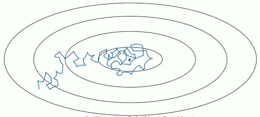
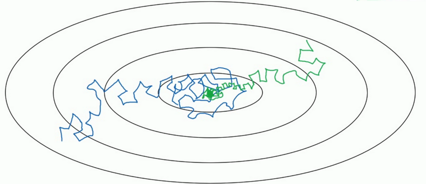
• 但如果能慢慢減少學習率 \(\alpha\) 的話,在初期的時候,你的學習率還比較大,能夠學習的很快,但是隨著 \(\alpha\) 變小,你的步伐也會變慢變小.所以最後的曲線在最小值附近的一小塊區域裏擺動.所以慢慢減少 \(\alpha\) 的本質在於在學習初期,你能承受較大的步伐, 但當開始收斂的時候,小一些的學習率能讓你的步伐小一些.

細節

• 一個epoch表示要遍歷一次數據,即就算有多個mini-batch,但是一定要遍歷所有數據一次,才叫做一個epoch.
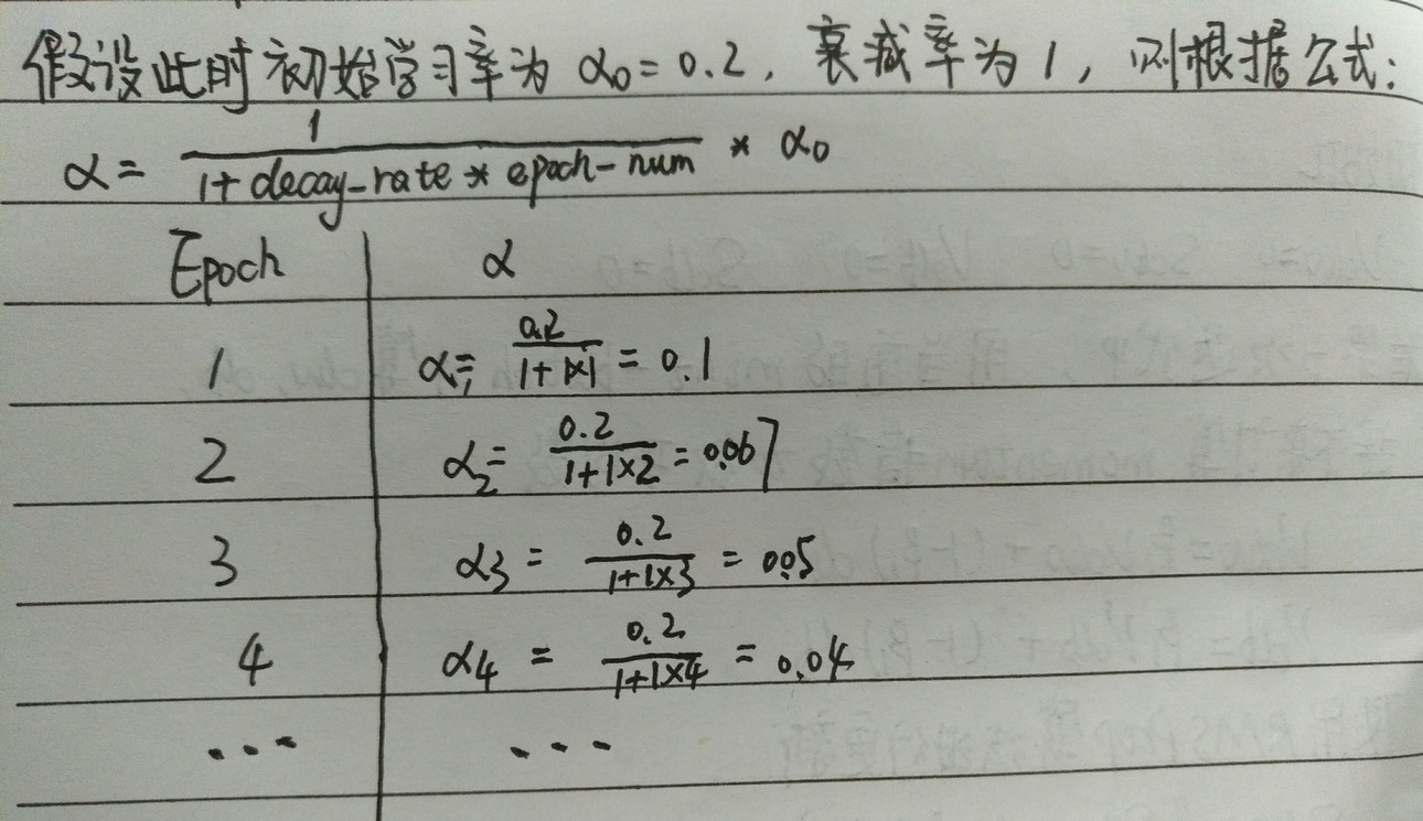
• 學習率 \(\alpha ,其中 \alpha_{0}表示初始學習率, decay-rate是一個新引入的超參數\)
  :
  \[\alpha = \frac{1}{1+decay-rate*epoch-num}*\alpha_{0}\]

其他學習率是衰減公式

指數衰減

\[\alpha = decay-rate^{epoch-num}*\alpha_{0}\]
\[\alpha = \frac{k}{\sqrt{epoch-num}}*\alpha_{0}其中k是超參數\]
\[\alpha = \frac{k}{\sqrt{t}}*\alpha_{0}其中k是超參數,t表示mini-batch的標記數字\]

Tensorflow實現學習率衰減

自適應學習率衰減

tf.train.exponential_decay(learning_rate, global_step, decay_steps, decay_rate, staircase=False, name=None)
退化學習率,衰減學習率,將指數衰減應用於學習速率。
計算公式:
decayed_learning_rate = learning_rate * decay_rate ^ (global_step / decay_steps)

# 初始的學習速率是0.1，總的叠代次數是1000次，如果staircase=True，那就表明每decay_steps次計算學習速率變化，更新原始學習速率，
# 如果是False，那就是每一步都更新學習速率。紅色表示False，藍色表示True。
import tensorflow as tf
import numpy as np
import matplotlib.pyplot as plt

learning_rate = 0.1  # 初始學習速率時0.1
decay_rate = 0.96  # 衰減率
global_steps = 1000  # 總的叠代次數
decay_steps = 100  # 衰減次數

global_ = tf.Variable(tf.constant(0))
c = tf.train.exponential_decay(learning_rate, global_, decay_steps, decay_rate, staircase=True)
d = tf.train.exponential_decay(learning_rate, global_, decay_steps, decay_rate, staircase=False)

T_C = []
F_D = []

with tf.Session() as sess:
   for i in range(global_steps):
       T_c = sess.run(c, feed_dict={global_: i})
       T_C.append(T_c)
       F_d = sess.run(d, feed_dict={global_: i})
       F_D.append(F_d)

plt.figure(1)
plt.plot(range(global_steps), F_D, ‘r-‘)# "-"表示折線圖,r表示紅色,b表示藍色
plt.plot(range(global_steps), T_C, ‘b-‘)
# 關於函數的值的計算0.96^(3/1000)=0.998
plt.show()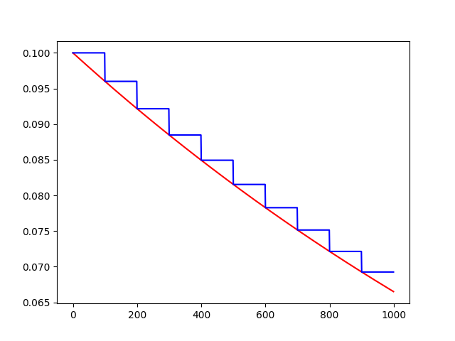

反時限學習率衰減

inverse_time_decay(learning_rate, global_step, decay_steps, decay_rate,staircase=False,name=None)
將反時限衰減應用到初始學習率。
計算公式：
decayed_learning_rate = learning_rate / (1 + decay_rate * t)

import tensorflow as tf
import matplotlib.pyplot as plt

global_ = tf.Variable(tf.constant(0), trainable=False)
globalstep = 10000  # 全局下降步數
learning_rate = 0.1  # 初始學習率
decaystep = 1000  # 實現衰減的頻率
decay_rate = 0.5  # 衰減率

t = tf.train.inverse_time_decay(learning_rate, global_, decaystep, decay_rate, staircase=True)
f = tf.train.inverse_time_decay(learning_rate, global_, decaystep, decay_rate, staircase=False)

T = []
F = []

with tf.Session() as sess:
    for i in range(globalstep):
        t_ = sess.run(t, feed_dict={global_: i})
        T.append(t_)
        f_ = sess.run(f, feed_dict={global_: i})
        F.append(f_)

plt.figure(1)
plt.plot(range(globalstep), T, ‘r-‘)
plt.plot(range(globalstep), F, ‘b-‘)
plt.show()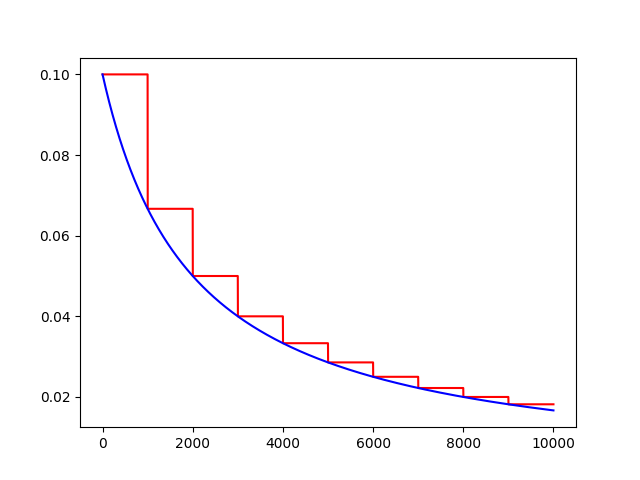

學習率自然指數衰減

def natural_exp_decay(learning_rate, global_step, decay_steps, decay_rate, staircase=False, name=None)
將自然指數衰減應用於初始學習速率。
計算公式:
decayed_learning_rate = learning_rate * exp(-decay_rate * global_step)

import tensorflow as tf
import matplotlib.pyplot as plt

global_ = tf.Variable(tf.constant(0), trainable=False)
globalstep = 10000  # 全局下降步數
learning_rate = 0.1  # 初始學習率
decaystep = 1000  # 實現衰減的頻率
decay_rate = 0.5  # 衰減率

t = tf.train.natural_exp_decay(learning_rate, global_, decaystep, decay_rate, staircase=True)
f = tf.train.natural_exp_decay(learning_rate, global_, decaystep, decay_rate, staircase=False)

T = []
F = []

with tf.Session() as sess:
    for i in range(globalstep):
        t_ = sess.run(t, feed_dict={global_: i})
        T.append(t_)
        f_ = sess.run(f, feed_dict={global_: i})
        F.append(f_)

plt.figure(1)
plt.plot(range(globalstep), T, ‘r-‘)
plt.plot(range(globalstep), F, ‘b-‘)
plt.show()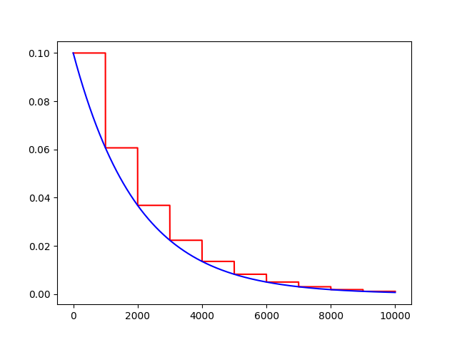

常數分片學習率衰減

piecewise_constant(x, boundaries, values, name=None)
例如前1W輪叠代使用1.0作為學習率，1W輪到1.1W輪使用0.5作為學習率，以後使用0.1作為學習率。

import tensorflow as tf
import numpy as np
import matplotlib.pyplot as plt

# 當global_取不同的值時learning_rate的變化，所以我們把global_
global_ = tf.Variable(tf.constant(0), trainable=False)
boundaries = [10000, 12000]
values = [1.0, 0.5, 0.1]
learning_rate = tf.train.piecewise_constant(global_, boundaries, values)
global_steps = 20000

T_L = []
with tf.Session() as sess:
    for i in range(global_steps):
        T_l = sess.run(learning_rate, feed_dict={global_: i})
        T_L.append(T_l)

plt.figure(1)
plt.plot(range(global_steps), T_L, ‘r-‘)
plt.show()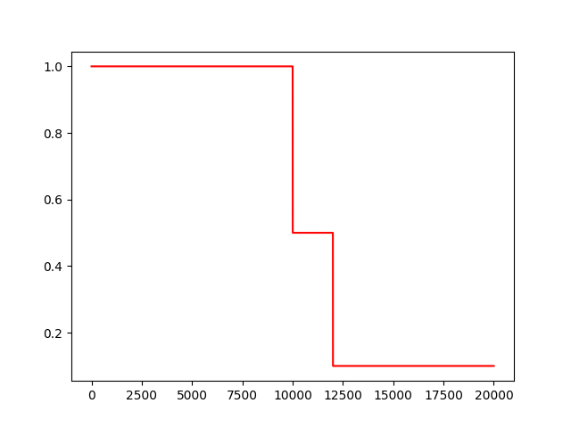

多項式學習率衰減

特點是確定結束的學習率。
polynomial_decay(learning_rate, global_step, decay_steps,end_learning_rate=0.0001, power=1.0,cycle=False, name=None):
通常觀察到，通過仔細選擇的變化程度的單調遞減的學習率會產生更好的表現模型。此函數將多項式衰減應用於學習率的初始值。
使學習率learning_rate在給定的decay_steps中達到end_learning_rate。它需要一個global_step值來計算衰減的學習速率。你可以傳遞一個TensorFlow變量，在每個訓練步驟中增加global_step = min(global_step, decay_steps)
計算公式:
decayed_learning_rate = (learning_rate - end_learning_rate) (1 - global_step / decay_steps) ^ (power) + end_learning_rate
如果cycle為True，則使用decay_steps的倍數，第一個大於‘global_steps`.ceil表示向上取整.
decay_steps = decay_steps ceil(global_step / decay_steps)
decayed_learning_rate = (learning_rate - end_learning_rate) *(1 - global_step / decay_steps) ^ (power) + end_learning_rate

Example: decay from 0.1 to 0.01 in 10000 steps using sqrt (i.e. power=0.5):‘‘‘
import tensorflow as tf
import matplotlib.pyplot as plt

global_ = tf.Variable(tf.constant(0), trainable=False)
starter_learning_rate = 0.1  # 初始學習率
end_learning_rate = 0.01  # 結束學習率
decay_steps = 1000
globalstep = 10000
f = tf.train.polynomial_decay(starter_learning_rate, global_, decay_steps, end_learning_rate, power=0.5, cycle=False)
t = tf.train.polynomial_decay(starter_learning_rate, global_, decay_steps, end_learning_rate, power=0.5, cycle=True)
F = []
T = []
with tf.Session() as sess:
    for i in range(globalstep):
        f_ = sess.run(f, feed_dict={global_: i})
        F.append(f_)
        t_ = sess.run(t, feed_dict={global_: i})
        T.append(t_)

plt.figure(1)
plt.plot(range(globalstep), F, ‘r-‘)
plt.plot(range(globalstep), T, ‘b-‘)
plt.show()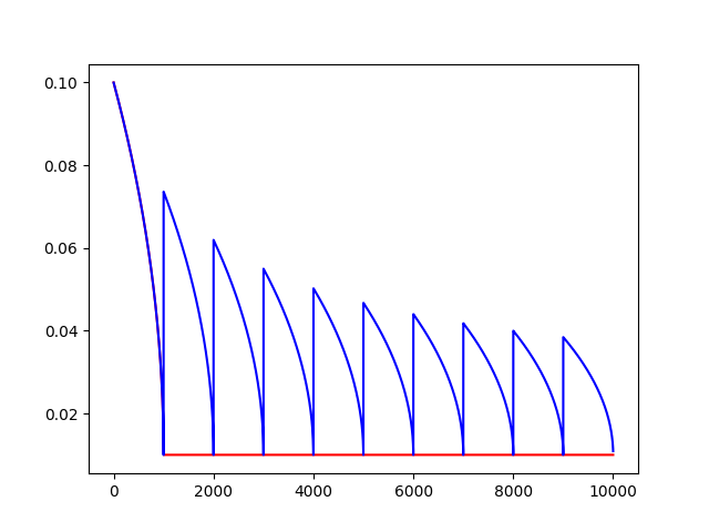

Tensorflow實現學習率衰減