吳恩達機器學習 - PCA演算法降維 吳恩達機器學習 - PCA演算法降維
阿新 • • 發佈:2018-11-05
原
吳恩達機器學習 - PCA演算法降維
2018年06月25日 13:08:17 離殤灬孤狼 閱讀數:152 更多<div class="tags-box space"> <span class="label">個人分類:</span> <a class="tag-link" href="https://blog.csdn.net/wyg1997/article/category/7742222" target="_blank">吳恩達機器學習 </a> </div> </div> <div class="operating"> </div> </div> </div> </div> <article> <div id="article_content" class="article_content clearfix csdn-tracking-statistics" data-pid="blog" data-mod="popu_307" data-dsm="post" style="height: 2070px; overflow: hidden;"> <div class="article-copyright"> 版權宣告:如果感覺寫的不錯,轉載標明出處連結哦~blog.csdn.net/wyg1997 https://blog.csdn.net/wyg1997/article/details/80800514 </div> <div class="markdown_views"> <!-- flowchart 箭頭圖示 勿刪 --> <svg xmlns="http://www.w3.org/2000/svg" style="display: none;"><path stroke-linecap="round" d="M5,0 0,2.5 5,5z" id="raphael-marker-block" style="-webkit-tap-highlight-color: rgba(0, 0, 0, 0);"></path></svg> <p>題目連結:<a href="https://s3.amazonaws.com/spark-public/ml/exercises/on-demand/machine-learning-ex7.zip" rel="nofollow" target="_blank">點選開啟連結</a></p>
筆記:
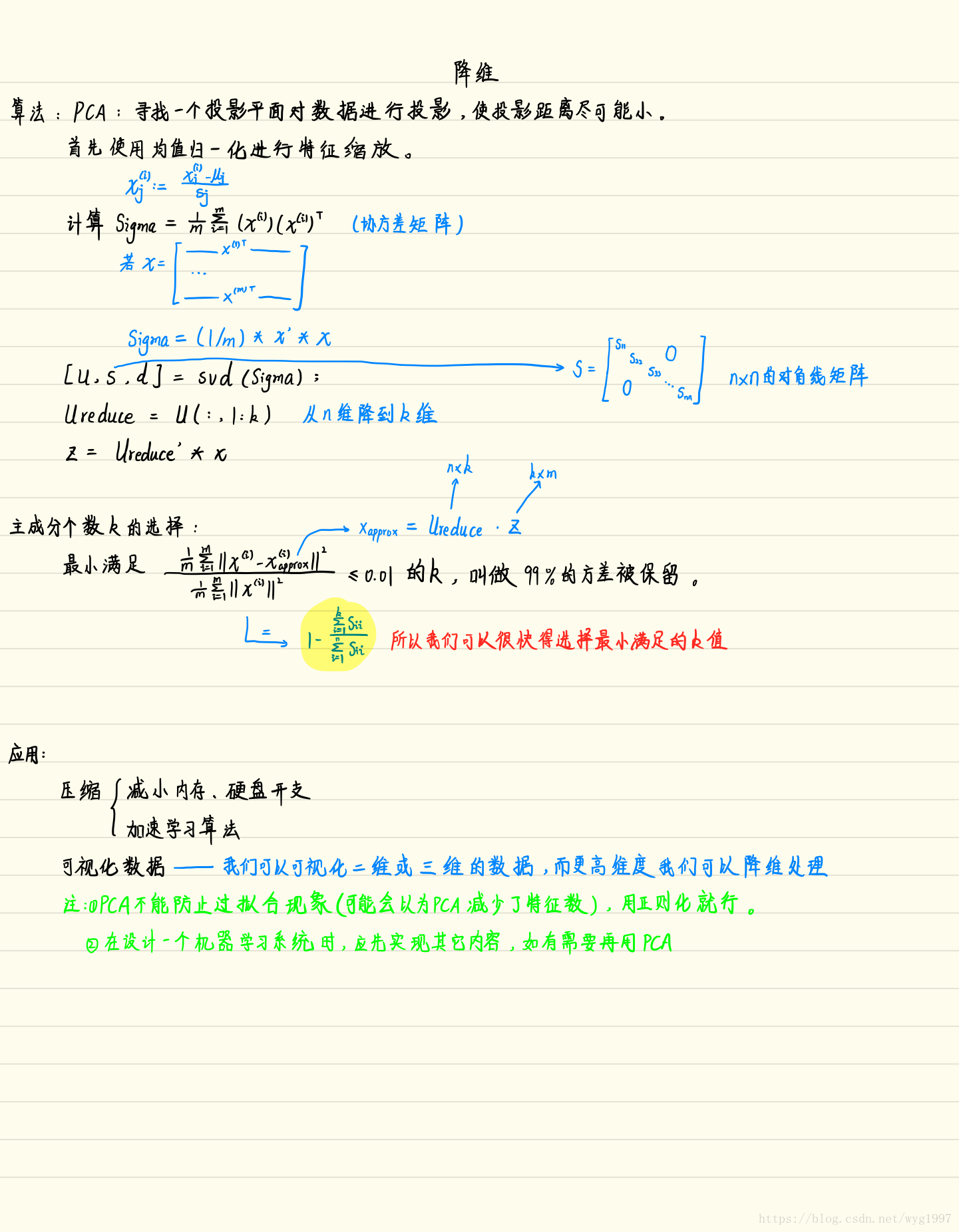
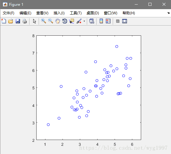
資料視覺化:
求矩陣U和S(pca.m):
function [U, S] = pca(X)
%PCA Run principal component analysis on the dataset X
% [U, S, X] = pca(X) computes eigenvectors of the covariance matrix of X
% Returns the eigenvectors U, the eigenvalues (on diagonal) in S
%
% Useful values
- 1
- 2
- 3
- 4
- 5
- 6
- 7
- 8
- 9
- 10
- 11
- 12
- 13
- 14
- 15
- 16
- 17
- 18
- 19
- 20
- 21
- 22
- 23
- 24
- 25
- 26
- 27
- 28
降維(projectData.m):
function Z = projectData(X, U, K)
%PROJECTDATA Computes the reduced data representation when projecting only
%on to the top k eigenvectors
%   Z = projectData(X, U, K) computes the projection of
%   the normalized inputs X into the reduced dimensional space spanned by
%   the first K columns of U. It returns the projected examples in Z.
%

% You need to return the following variables correctly.
Z = zeros(size(X, 1), K);

% ====================== YOUR CODE HERE ======================
% Instructions: Compute the projection of the data using only the top K
%               eigenvectors in U (first K columns).
%               For the i-th example X(i,:), the projection on to the k-th
%               eigenvector is given as follows:
%                    x = X(i, :)';
%                    projection_k = x' * U(:, k);
%

U_reduce = U(:,1:K);
Z = X*U_reduce;

% =============================================================

end
- 1
- 2
- 3
- 4
- 5
- 6
- 7
- 8
- 9
- 10
- 11
- 12
- 13
- 14
- 15
- 16
- 17
- 18
- 19
- 20
- 21
- 22
- 23
- 24
- 25
- 26
壓縮重現(投影后的位置)(recoverData.m):
function X_rec = recoverData(Z, U, K)
%RECOVERDATA Recovers an approximation of the original data when using the
%projected data
%   X_rec = RECOVERDATA(Z, U, K) recovers an approximation the
%   original data that has been reduced to K dimensions. It returns the
%   approximate reconstruction in X_rec.
%

% You need to return the following variables correctly.
X_rec = zeros(size(Z, 1), size(U, 1));

% ====================== YOUR CODE HERE ======================
% Instructions: Compute the approximation of the data by projecting back
%               onto the original space using the top K eigenvectors in U.
%
%               For the i-th example Z(i,:), the (approximate)
%               recovered data for dimension j is given as follows:
%                    v = Z(i, :)';
%                    recovered_j = v' * U(j, 1:K)';
%
%               Notice that U(j, 1:K) is a row vector.
%

X_rec = Z*U(:,1:K)';

% =============================================================

end
- 1
- 2
- 3
- 4
- 5
- 6
- 7
- 8
- 9
- 10
- 11
- 12
- 13
- 14
- 15
- 16
- 17
- 18
- 19
- 20
- 21
- 22
- 23
- 24
- 25
- 26
- 27
- 28
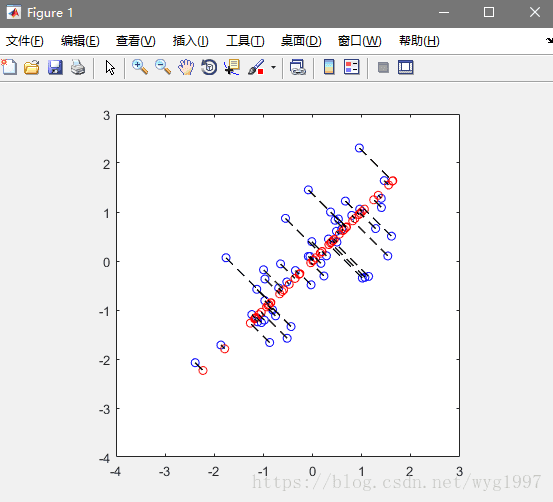
效果圖:
然後是兩個應用了
第一個是人臉資料的壓縮,可以加速其它的學習演算法
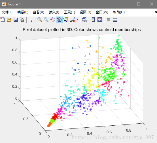
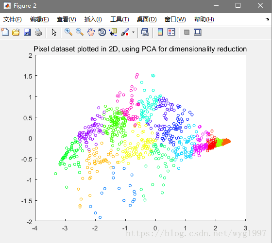
第二個是資料視覺化,把一個3D的資料壓縮到2D上看的更清楚
如圖: