linear regression

This is my study notes in machine learning, writing articles in English because I want to improve my writing skills. Anyway, thanks for watching and if I made some mistakes, let me know please.

The objective of linear algebra is to calculate relationships of points in vector space.

Simple linear regression is used to find the best fit line of a dataset. If the data isn’t continuous, there really isn’t going to be a best fit line.

During our model, the X coordinates are the features and the Y coordinates are the associated labels.

Here is a simple straight line: y = mx + b

Least squares

The method of least squares is a standard and useful approach in regression analysis to approximate the solution.
The important application is in data fitting, which means there are many points spread in diagram, we may find a best-fit line y = mx + b

What least squares means?

overall solutions minimizes the sum of the squares of the residuals made in the results of every single equation.

So, during data fitting, we should minimizes the sum of squared residuals which means minimizes the difference between observed values and fitted value provided by model.Linear regression is one kind of data fitting.

However, least squares have problem in some case with substantial uncertainties in independent variable, use errors-in-variables models to instead.

Two kinds of least squares problems depending residuals are linear or not:

• linear or ordinary least squares
• nonlinear least squares

Besides, while solving nonlinear problems usually try to use a linear function to approximate it in each iterative, the core calculation is so similar.

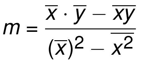
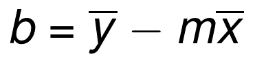
How to calculate m and b?
From y = mx + b, in general is y = mx + b + e, e represent errors. In this case, our objective is to find out (m,b) which makes the difference between our predicted value(fitted value) and the real value(observed value). We decide the square loss function: $L_n = (y_n-(x_m+b))^2$
So, mean loss overall data sets is: $L = \frac 1N\sum_{n=1}^NL_n$
$L = \frac 1N\sum_{n=1}^N(y_n^2-2y_nb+2mx_n(b-y_n)+b^2+m^2x_n^2)$

Now, for minimizing square loss function $L$, makes partial derivative of $L$ with respect to $m$ and $b$ equal $0$ which leads the derivative of $L$ equal $0$, it means this parameter of $(m,b)$ is the best.

Take all items without $b$ out:
$\frac 1N\sum_{n=1}^N(b^2-2y_n b+2mbx_n)$ $\frac {\partial L}{\partial b}=2b-\frac 2N\sum_{n=1}^Ny_n+\frac {2m}N\sum_{n=1}^Nx_n$
Take all items without $m$ out:
$\frac 1N\sum_{n=1}^N(2mx_n(b-y_n)+m^2x_n^2)$ $\frac {\partial L}{\partial m}=\frac 2N\sum_{n=1}^Nx_n(b-y_n)+\frac {2m}N\sum_{n=1}^N x_n^2$
Finally, let $\frac {\partial L}{\partial m}=0$ and $\frac {\partial L}{\partial b}=0$, we can calculate the solution.