
機器學習之Scipy庫
1.1 總體說明
SciPy是一款方便、易於使用、專為科學和工程設計的Python工具包。它包括統計、優化、涉及線性代數模組、傅立葉變換、訊號和影象處理、常微分方程求解器等眾多數學包。
1.2 代表性函式使用介紹
1.最優化
(1)資料建模和擬合
SciPy函式curve_fit使用基於卡方的方法進行線性迴歸分析。下面,首先使用f(x)=ax+b生成帶有噪聲的資料,然後使用curve_fit來擬合。
例如:線性迴歸
import numpy as np
from scipy.optimize import curve_fit
#建立函式f(x) = ax + b
def func(x,a,b):
    return a*x+b

#建立乾淨資料
x = np.linspace(0,10,100)
y = func(x,1,2)

#新增噪聲
yn = y + 0.9* np.random.normal(size=len(x))

#擬合噪聲資料
popt,pcov = curve_fit(func,x,yn)

#輸出最優引數
print(popt)

例如:高斯分佈擬合
#建立函式
def func(x,a,b,c):
    return a*np.exp(-(x-b)**2/(2*c**2))

#生成乾淨資料
x = np.linspace(0,10,100)
y = func(x,1,5,2)

#新增噪聲
yn = y+0.2*np.random.normal(size=len(x))

#擬合
popt,pcov = curve_fit(func,x,yn)

print(popt)

(2)函式求解
SciPy的optimize模組中有大量的函式求解工具,fsolve是其中最常用的
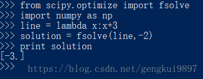
例如:線性函式求解
from scipy.optimize import fsolve
import numpy as np
line = lambda x:x+3
solution = fsolve(line,-2)
print solution
例如:求函式交叉點
from scipy.optimize import fsolve
import numpy as np

#用於求解的解函式
def findIntersection(func1,func2,x0):
    return fsolve(lambda x : func1(x)-func2(x),x0)

#兩個函式
funky = lambda x :np.cos(x/5)*np.sin(x/2)
line = lambda x : 0.01*x - 0.5
x = np.linspace(0,45,10000)
result = findIntersection(funky,line,[15,20,30,35,40,45])

#輸出結果
print(result,line(result))

2.插值
(1)interp1d
例如:正弦函式插值
import numpy as np
from scipy.interpolate import interp1d

#建立待插值的資料
x = np.linspace(0,10*np.pi,20)
y = np.cos(x)

#分別用linear和quadratic插值
fl = interp1d(x,y,kind='linear')
fq = interp1d(x,y,kind='quadratic')
xint = np.linspace(x.min(),x.max(),1000)
yintl = fl(xint)
yintq = fq(xint)
(2)UnivariateSpline
例如:噪聲資料插值
import numpy as np
from scipy.interpolate import UnivariateSpline

#建立含噪聲的待插值資料
sample = 30
x = np.linspace(1,10*np.pi,sample)
y = np.cos(x) + np.log10(x) + np.random.randn(sample)/10

#插值,引數s為smoothing factor
f = UnivariateSpline(x,y,s=1)
xint = np.linspace(x.min(),x.max(),1000)
yint = f(xint)
(3)griddata
例如:利用插值重構圖片
import numpy as np
from scipy.interpolate import griddata

#定義一個函式
ripple = lambda x,y : np.sqrt(x**2+y**2) + np.sin(x**2,y**2)

#生成grid資料,複數定義了生成grid資料的step,若無該複數則step為5
grid_x,grid_y = np.mgrid[0:5:1000j,0:5:1000j]

#生成待插值的資料樣本
xy = np.random.rand(1000,2)
sample = ripple(xy[:,0]*5,xy[:,1]*5)

#用cubic方法插值
grid_z0 = griddata(xy*5,sample,(grid_x,grid_y),method='cubic')
(4)SmoothBivariateSpline
例如:利用插值重構圖片
import numpy as np
from scipy.interpolate import SmoothBivariateSpline as SBS

#定義函式
ripple = lambda x,y : np.sqrt(x**2+y**2)+np.sin(x**2+y**2)

#生成待插值樣本
xy=np.random.rand(1000,2)
x,y = xy[:,0],xy[:,1]
sample = ripple(xy[:,0]*5,xy[:,1]*5)

#插值
fit = SBS(x*5,y*5,sample,s=0.01,kx=4,ky=4)
interp = fit(np.linspace(0,5,1000),np.linspace(0,5,1000))
3.積分
(1)解析積分
import numpy as np
from scipy.integrate import quad

#定義被積函式
func = lambda x:np.cos(np.exp(x))**2

#積分
solution = quad(func,0,3)
print solution
(2)數值積分
import numpy as np
from scipy.integrate import quad,trapz

x = np.sort(np.random.randn(150)*4+4).clip(0,5)
func = lambda x:np.sin(x)*np.cos(x**2)+1
y = func(x)

fsolution = quad(func,0,5)
dsolution = trapz(y,x=x)
print('fsolution='+str(fsolution[0]))
print('dsolution='+str(dsolution))
print('The difference is '+str(np.abs(fsolution[0]-dsolution)))
4.統計
SciPy中包括mean,std,median,argmax及argmin等在內的基本統計函式,而且numpy.arrays型別中內建了大部分統計函式,以便易於使用。
import numpy as np
elements x = np.random.randn(1000)
mean = x.mean() #均值
std = x.std() #標準差
var = x.var() #方差
SciPy中還包括了各種分佈、函式等工具。連續和離散分佈SciPy的scipy.stats包中包含了大概80種連續分佈和10種離散分佈。
例如:概率密度函式(PDFs)
import numpy as np
from scipy.stats import norm

#建立樣本區間
x = np.linspace(-5,5,1000)

#設定正態分佈引數,loc為均值,scale為標準差
dist = norm(loc=0,scale=1)

#得到正態分佈的PDF和CDF
pdf = dist.pdf(x)
cdf = dist.cdf(x)

#根據分佈生成500個隨機數
sample = dist.rvs(500)
例如:幾何分佈概率分佈函式(PMF)
import numpy as np
from scipy.stats import geom

#設定幾何分佈引數
p = 0.5
dist = geom(p)

#設定樣本空間
x = np.linspace(0,5,1000)

#得到幾何分佈的PMF和CDF
pmf = dist.pmf(x)
cdf = dist.cdf(x)

#生成500個隨機數
sample = dist.rvs(500)
例如:樣本分佈檢驗
import numpy as np
from scipy import stats

#生成包括100個服從正態分佈的隨機數樣本
sample = np.random.randn(100)

#用normaltest檢驗原假設
out = stats.normaltest(sample)
print('normaltest output')
print('Z-score = '+str(out[0]))
print('P-value = '+str(out[1]))

#ktest是檢驗擬合度的kolmogorov-Smirnov檢驗,這裡針對正態分佈進行檢驗
#D是KS統計量的值,越接近0越好
out = stats.kstest(sample,'norm')
print('\nkstest output for the Normal distribution')
print('D = '+str(out[0]))
print('P-value = '+str(out[1]))

#類似地可以針對其他分佈進行檢驗,如Wald分佈
out = stats.kstest(sample,'wald')
print('\nkstest output for the Wald distribution')
print('D = '+str(out[0]))
print('P-value = '+str(out[1]))
5.空間和聚類分析
(1)向量量化
向量量化是訊號處理、資料壓縮和聚類等領域通用的術語。這裡僅關注其在聚類中的應用
例如:k均值聚類
import numpy as np
from scipy.cluster import vq

#生成資料
c1 = np.random.randn(100,2)+5
c2 = np.random.randn(30,2)-5
c3 = np.random.randn(50,2)

#將所有資料放入一個180*2的陣列
data = np.vstack([c1,c2,c3])

#利用k均值方法計算聚類的質心和方差
centroids,variance = vq.kmeans(data,3)

#變數identified中存放關於聚類的資訊
identified,distance = vq.vq(data,centroids)

#獲得各類別的資料
vqc1 = data[identified == 0]
vqc2 = data[identified == 1]
vqc3 = data[identified == 2]
(2)層次聚類
層次聚類是一種重要的聚類方法,但其輸出結果比較複雜,不能像k均值那樣給出清晰的聚類結果。
例如:輸入一個距離矩陣,輸出一個樹狀圖
#coding:utf-8
import numpy as np
import matplotlib.pyplot as mpl
from scipy.spatial.distance import pdist,squareform
import scipy.cluster.hierarchy as hy

#用於生成聚類資料的函式
def clusters(number=20,cnumber=5,csize=10):
    #聚類服從高斯分佈
    rnum = np.random.rand(cnumber,2)
    rn = rnum[:,0]*number
    rn = rn.astype(int)
    rn[np.where(rn<5)] = 5
    rn[np.where(rn>number/2.)] = round(number/2.0)
    ra = rnum[:,1]*2.9
    ra[np.where(ra<1.5)] = 1.5
    cls = np.random.randn(number,3)*csize
    rxyz = np.random.randn(cnumber-1,3)
    for i in xrange(cnumber-1):
        tmp = np.random.randn(rn[i+1],3)
        x = tmp[:,0]+(rxyz[i,0]*csize)
        y = tmp[:,1]+(rxyz[i,1]*csize)
        z = tmp[:,2]+(rxyz[i,2]*csize)
        tmp = np.column_stack([x,y,z])
        cls = np.vstack([cls,tmp])
    return cls

#建立待聚類資料及距離矩陣
cls = clusters()
D = pdist(cls[:,0:2])
D = squareform(D)

#繪製左側樹狀圖
fig = mpl.figure(figsize=(8,8))
ax1 = fig.add_axes([0.09,0.1,0.2,0.6])
Y1 = hy.linkage(D,method='complete')
cutoff = 0.3 * np.max(Y1[:,2])
Z1 = hy.dendrogram(Y1,orientation='left',color_threshold=cutoff)
ax1.xaxis.set_visible(False)
ax1.yaxis.set_visible(False)

#繪製頂部樹狀圖
ax2 = fig.add_axes([0.3,0.71,0.6,0.2])
Y2 = hy.linkage(D,method='average')
cutoff = 0.3 * np.max(Y2[:,2])
Z2 = hy.dendrogram(Y2,color_threshold=cutoff)
ax2.xaxis.set_visible(False)
ax2.yaxis.set_visible(False)

#顯示距離矩陣
ax3 = fig.add_axes([0.3,0.1,0.6,0.6])
idx1 = Z1['leaves']
idx2 = Z2['leaves']
D = D[idx1,:]
D = D[:,idx2]
ax3.matshow(D,aspect='auto',origin='lower',cmap=mpl.cm.YlGnBu)
ax3.xaxis.set_visible(False)
ax3.yaxis.set_visible(False)

#儲存圖片,顯示圖片
fig.savefig('cluster_hy_f01.pdf',bbox='tight')
mpl.show()

在上圖雖然計算了資料點之間的距離,但是還是難以將各類·區分開。函式fcluster可以根據閾值來區分各類,其輸出結果依賴於linkage函式所採用的方法,如complete或者single等,它的第二個引數既是閾值。dendrogram函式中預設的閾值是0.7*np.max(Y[:,2]),這裡還使用0.3。
例如:
#coding:utf-8
import numpy as np
import matplotlib.pyplot as mpl
from scipy.spatial.distance import pdist,squareform
import scipy.cluster.hierarchy as hy

#得到不同類別資料點的座標
def group(data,index):
    number = np.unique(index)
    groups = []
    for i in number:
        groups.append(data[index == i])
    return groups

#用於生成聚類資料的函式
def clusters(number=20,cnumber=5,csize=10):
    #聚類服從高斯分佈
    rnum = np.random.rand(cnumber,2)
    rn = rnum[:,0]*number
    rn = rn.astype(int)
    rn[np.where(rn<5)] = 5
    rn[np.where(rn>number/2.)] = round(number/2.0)
    ra = rnum[:,1]*2.9
    ra[np.where(ra<1.5)] = 1.5
    cls = np.random.randn(number,3)*csize
    rxyz = np.random.randn(cnumber-1,3)
    for i in xrange(cnumber-1):
        tmp = np.random.randn(rn[i+1],3)
        x = tmp[:,0]+(rxyz[i,0]*csize)
        y = tmp[:,1]+(rxyz[i,1]*csize)
        z = tmp[:,2]+(rxyz[i,2]*csize)
        tmp = np.column_stack([x,y,z])
        cls = np.vstack([cls,tmp])
    return cls

#建立資料
cls = clusters()

#計算linkage矩陣
Y = hy.linkage(cls[:,0:2],method='complete')

#從層次資料結構中,用fcluster函式將層次結構的資料轉為flat cluster
cutoff = 0.3 * np.max(Y[:,2])
index = hy.fcluster(Y,cutoff,'distance')

#使用groups函式將資料劃分類別
groups = group(cls,index)

#繪製資料點
fig = mpl.figure(figsize=(6,6))
ax = fig.add_subplot(111)
colors = ['r','c','b','g','orange','k','y','gray']
for i,g in enumerate(groups):
    i = np.mod(i,len(colors))
    ax.scatter(g[:,0],g[:,1],c=colors[i],edgecolor='none',s=50)
    ax.xaxis.set_visible(False)
    ax.yaxis.set_visible(False)

fig.savefig('cluster_hy_f02.pdf',bbox='tight')
mpl.show()
6.稀疏矩陣
NumPy處理10^6級別的資料沒有什麼大問題·,當資料量達到10^7級別時速度開始變慢,記憶體受到限制。當處理超大規模資料集,比如10^10級別,且資料中包含大量的0時,可採用稀疏矩陣提高速度和效率
提示:使用data.nbytes可檢視資料可佔空間大小
例如:矩陣與稀疏矩陣運算對比
# coding:utf-8
import numpy as np
from scipy.sparse.linalg import eigsh
from scipy.linalg import eigh
import scipy.sparse
import time

N = 3000

#建立隨機稀疏矩陣
m = scipy.sparse.rand(N,N)

#建立包含相同資料的陣列
a = m.toarray()
print('The numpy array data size: '+str(a.nbytes)+' bytes')
print('The sparse matrix data size: '+str(m.data.nbytes)+' bytes')

#陣列求特徵值
t0 = time.time()
res2 = eigh(a)
dt = str(np.round(time.time()-t0,3))+' seconds'
print('Non-sparse operation takes '+dt)

#稀疏矩陣求特徵值
t0 = time.time()
res2 = eigsh(m)
dt = str(np.round(time.time()-t0,3)) + ' seconds'
print('Sparse operation takes '+dt)
