
[Computer Vision][IMAGE FORMATION] 1 Geometric Camera Models 1.2 PARAMETERS(2)
目錄
弱透視模型的座標變換和相機引數
我們按照和上一節類似的思路來推導弱透視模型的座標變換公示,並給出這種情況下的相機引數。
1 從世界座標系到相機座標系
這一步和之前一樣,得到:

2 從相機座標系到投影座標系
在這一步中,我們忽略了物體的厚度。通常的做法是在物體上取一個參考點,過這個參考點作光軸的垂面,然後將其他點都投影到這個平面上。即認為所有點的Z座標都與參考點的相等。不妨設這一座標值為Zr,於是得到投影座標:
p = (f/Zr X, f/Zr Y, 1) = f/Zr = f/Zr
P
3 從投影座標系到螢幕座標系
這一步和上一節的一般情況下的做法相同,使用K來完成轉換(注意係數f包含在K中),最終的表示式為:
=
 = MPw。
注意到的秩為2,也就是說,我們可以將表示式化簡。記:
 ,其中
,其中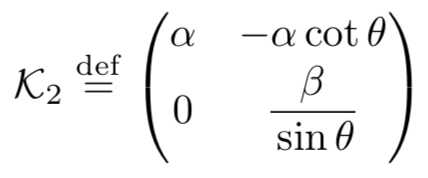 ,
, ;
;
R2 = ,t2 =
。
於是:
M =
=
=
=
=
=。
由於我們實際上並不需要齊次座標系中的最後一個座標,所以可以丟掉第三行,取:
,
得到的表示式
= MPw。
4 變數的耦合問題
在上面的推導中,我們注意到一個現象:令t2 = t2 + a,p0 = p0 - 1/Zr K2a,M並不會改變。我們將這種現象稱為變數的耦合,本質上其實是一種資訊的丟失。具體來說,如果我們換一個相機,它的t變數的前兩維是t2 + a,主點在畫素座標系上的座標是p0 - 1/Zr K2a,我們得到的座標轉換的矩陣和之前的相機是相同的,也就是對同一個場景會得到相同的照片,這樣我們就無法區別這兩個相機,也就是無法唯一確定其中的一些引數。
此外,Zr和K2中的引數之間也存在這種變數耦合的問題:
1/Zr K = ,
其中和
總是分別作為整體出現,因而實際上也只能確定兩個自由度。從實際意義來看就是如果物點的距離更遠,同時CCD上的單位長度畫素數量或者焦距按相同比例放大,則我們得到的數字影象同樣不會改變。
事實上,我們在上一節即一般情形下,也遇到了一組變數耦合,即k、l和f的耦合。由於kf、lf總是以單項式的形式出現,我們將它們分別記作α和β,也就是隻能確定兩個自由度。
根據這種情況,我們可以進一步簡化M的引數:
M =
= (根據之前的結論,p0可以任意選取,此時的t2也被更新了)
= (按照分塊矩陣乘法計算即可)
=
=
=
這時再來清點我們的變數,一共有八個:Zr是結構(structure)引數,k、s是與CCD的畸變程度和畫素密度相關的引數,t2中包含了兩個引數,R2雖然只有兩行,但是寫出R的實際形式可以看出R2中仍然存在三個角度引數。