
反向傳播演算法(BP演算法)
BP演算法(即反向傳播演算法),適合於多層神經元網路的一種學習演算法,它建立在梯度下降法的基礎上。BP網路的輸入輸出關係實質上是一種對映關係:一個n輸入m輸出的BP神經網路所完成的功能是從n維歐氏空間向m維歐氏空間中一有限域的連續對映,這一對映具有高度非線性。它的資訊處理能力來源於簡單非線性函式的多次複合,因此具有很強的函式復現能力。這是BP演算法得以應用的基礎。
反向傳播演算法主要由兩個環節(激勵傳播、權重更新)反覆迴圈迭代,直到網路的對輸入的響應達到預定的目標範圍為止。
由一個數據算出得分值這個過程叫做前向傳播,由一個得分值算出loss值,再有loss值往回傳,什麼樣的w該更新,什麼樣的w該更新多大的值這個過程叫做反向傳播。在反向傳播的過程中最重要的是更新權重引數W。
下面我們用一個例項來說明:
如下圖所示:
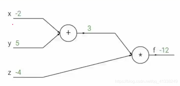
上圖表示有三個樣本點下x,y,z
1.對x和y進行求和操作
2.將x和y求出的和和z求乘積
f(x,y,z)=(x+y)*Z
例如我們分別給x,y,z賦值為-2,5,-4那麼我們得出的f=-12
那麼我們好比f就等於損失值為-12
得出損失值後我們要求x,y,z分別對f做出了多大的貢獻
我們指定一個q=x+y對第一個節點進行操作
此時f=q*z
如果我們求z對f做了多少影響,只需對z進行求偏導值為3,意思就是如果z增大1倍,那麼f值就會增大3倍
如果我們求q對f做了多少影響,只需對q進行求偏導值為-4,意思就是如果q增大1倍,那麼f值就會減少4倍
如圖所示: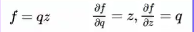
如果我們求x對f做了多大的貢獻,那麼我們先要求x對q做了多大的貢獻,求對x求偏導如圖所示:
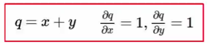
q對f做的貢獻為-4,所以x對f的貢獻為1*(-4)為-4,這個過程稱作為鏈式法則
我們的梯度要根據鏈式法則一層一層的往下傳。這樣我們就能更新我們的權重引數。
上面這個例子形象的講解了反向傳播的過程和如何實現權重的更新。
下面用程式碼實現:
import numpy as np

# "pd" 偏導
def sigmoid(x):
    return 1 / (1 + np.exp(-x))
def sigmoidDerivationx(y):
    return y * (1 - y)

if __name__ == "__main__":
    #初始化
    bias = [0.35, 0.60]
    weight = [0.15, 0.2, 0.25, 0.3, 0.4, 0.45, 0.5, 0.55]
    output_layer_weights = [0.4, 0.45, 0.5, 0.55]
    i1 = 0.05
    i2 = 0.10
    target1 = 0.01
    target2 = 0.99
    alpha = 0.5 #學習速率
    numIter = 90000 #迭代次數
    for i in range(numIter):
        #正向傳播
        neth1 = i1*weight[1-1] + i2*weight[2-1] + bias[0]
        neth2 = i1*weight[3-1] + i2*weight[4-1] + bias[0]
        outh1 = sigmoid(neth1)
        outh2 = sigmoid(neth2)
        neto1 = outh1*weight[5-1] + outh2*weight[6-1] + bias[1]
        neto2 = outh2*weight[7-1] + outh2*weight[8-1] + bias[1]
        outo1 = sigmoid(neto1)
        outo2 = sigmoid(neto2)
        print(str(i) + ", target1 : " + str(target1-outo1) + ", target2 : " + str(target2-outo2))
        if i == numIter-1:
            print("lastst result : " + str(outo1) + " " + str(outo2))
        #反向傳播
        #計算w5-w8(輸出層權重)的誤差
        pdEOuto1 = - (target1 - outo1)
        pdOuto1Neto1 = sigmoidDerivationx(outo1)
        pdNeto1W5 = outh1
        pdEW5 = pdEOuto1 * pdOuto1Neto1 * pdNeto1W5
        pdNeto1W6 = outh2
        pdEW6 = pdEOuto1 * pdOuto1Neto1 * pdNeto1W6
        pdEOuto2 = - (target2 - outo2)
        pdOuto2Neto2 = sigmoidDerivationx(outo2)
        pdNeto1W7 = outh1
        pdEW7 = pdEOuto2 * pdOuto2Neto2 * pdNeto1W7
        pdNeto1W8 = outh2
        pdEW8 = pdEOuto2 * pdOuto2Neto2 * pdNeto1W8
        # 計算w1-w4(輸出層權重)的誤差
        pdEOuto1 = - (target1 - outo1) #之前算過
        pdEOuto2 = - (target2 - outo2)  #之前算過
        pdOuto1Neto1 = sigmoidDerivationx(outo1)    #之前算過
        pdOuto2Neto2 = sigmoidDerivationx(outo2)    #之前算過
        pdNeto1Outh1 = weight[5-1]
        pdNeto1Outh2 = weight[7-1]
        pdENeth1 = pdEOuto1 * pdOuto1Neto1 * pdNeto1Outh1 + pdEOuto2 * pdOuto2Neto2 * pdNeto1Outh2
        pdOuth1Neth1 = sigmoidDerivationx(outh1)
        pdNeth1W1 = i1
        pdNeth1W2 = i2
        pdEW1 = pdENeth1 * pdOuth1Neth1 * pdNeth1W1
        pdEW2 = pdENeth1 * pdOuth1Neth1 * pdNeth1W2
        pdNeto1Outh2 = weight[6-1]
        pdNeto2Outh2 = weight[8-1]
        pdOuth2Neth2 = sigmoidDerivationx(outh2)
        pdNeth1W3 = i1
        pdNeth1W4 = i2
        pdENeth2 = pdEOuto1 * pdOuto1Neto1 * pdNeto1Outh2 + pdEOuto2 * pdOuto2Neto2 * pdNeto2Outh2
        pdEW3 = pdENeth2 * pdOuth2Neth2 * pdNeth1W3
        pdEW4 = pdENeth2 * pdOuth2Neth2 * pdNeth1W4
        #權重更新
        weight[1-1] = weight[1-1] - alpha * pdEW1
        weight[2-1] = weight[2-1] - alpha * pdEW2
        weight[3-1] = weight[3-1] - alpha * pdEW3
        weight[4-1] = weight[4-1] - alpha * pdEW4
        weight[5-1] = weight[5-1] - alpha * pdEW5
        weight[6-1] = weight[6-1] - alpha * pdEW6
        weight[7-1] = weight[7-1] - alpha * pdEW7
        weight[8-1] = weight[8-1] - alpha * pdEW8
        # print(weight[1-1])
        # print(weight[2-1])
        # print(weight[3-1])
        # print(weight[4-1])
        # print(weight[5-1])
        # print(weight[6-1])
        # print(weight[7-1])
        # print(weight[8-1])
BP演算法python實現參考https://blog.csdn.net/tudaodiaozhale/article/details/78632931