參考 ： https://www.scratchapixel.com/lessons/mathematics-physics-for-computer-graphics/monte-carlo-methods-mathematical-foundations

Sampling Distribution

In statistics when some characteristic(特性) of a given population can be calculated using all the elements(元素) or items in this

population, we say that the resulting value is a parameter(引數) of the population. The population mean for example is a

population parameter which is used to define the average value of a quantity. Parameters are fixed values. On the other hand,

when the we use samples to get an estimation

samples is a statistic(統計數值).

（a population parameter 定義：使用population的所有的資料去計算的一個值，例如 population mean

statisitic 定義，如果我們用取樣點去 估算 一個 a population parameter，那麼 這個估算值其實就是 statistic ）

As you can see in figure 3 the population generated by our program has an arbitrary distribution. This population is not

distributed accordining to any particular probability distribution,and espcially(尤其) not a normal distribution. The reason why

we made this choice will become clear very soon(很快就變得清晰). Because the distribution is discrete(離散) and finite(有限),

this population of course has a well defined mean and variance which we already computed above. What we are going to do

now is take a sample of size n from this population, compute its sample mean and repeat this experiment 1000 times. The

sample mean value will be rounded off(四捨五入) to the nearest integer value (so that it takes any integer value between 0 and

20). At the end of the process, we will count the number of samples whose means are either 0, or 1, or 2, ... up to 20. Figure 4

shows the results. Quite remarkably(十分明顯), as you can see, the distribution of samples follows a normal distribution. This is

not the distribution of cards here that we are looking at but the distribution of samples. Be sure to understand that difference

quite clearly. It is a distribution of statistics. Note also that this is not a perfect normal distribution (you know understand why

we have been very specific(特殊) about this in the previous chapter) because clearly, there is some difference between the

results and a perfect normal distribution (curve in red). In conclusion(最後), even thouh the distribution of the population is

arbitrary, the distribution of samples or statistics is not (but it converges in distribution to the normal distribution. We will come

back to this idea later).

（圖3表示的就是，標有數字【0-20】的卡片 與 個數 的分佈圖，圖4表示的意思就是，從這堆卡片中去抽取一張卡片，然後計算它的平均值(平均值經過四捨五入)，抽取1000次，記錄1000次的平均值，結果顯示，平均值的 分佈圖 像1個 normal distribution）

 In other words, instead of studying for example how the height (the property) of all adults from a given country (the population)

are distributed, we take samples from this population to estimate the population's average height, and look at how these

samples are distributed with regards to(關於) each other. In statistic, the distribution of samples (or statistics) is called

a sampling distribution. Similarly to the case of a population distribution, sampling distributions can be defined using models

(i.e. probability distributions). It defines how all possible samples are distributed for a given population and samples of a

given size.

Note 2: the sampling distribution of a statistic is the distribution of that statistic(統計數值), considered as a random variable,

when derived from(來源於) a random sample of size n. In other words, the sampling distribution of the mean is a distribution of

samples means.

Extend

First off(首先), you start with a population. Then you draw elements from this population randomly. In this particular diagram in

each experiment(試驗) we make what we call 3 observations(觀察值), in other words we draw 3 items from the population.

Because these are random variables, but possible outcomes from the experiment we label them with the lower case x. If now

take the weighted average of these 3 drawn items, we get what we call a statistic or sample whose size is n=3. To compute the

value of this sample, we use the equation for the expected value (or mean). Each sample on its own, is a random variable, but

because now they represent the mean of certain number n of items in the population, we label them with the upper letter X. We

can repeat this experiment N times which gives as series of samples: X1,X2,...XN. This collection(收集) of samples is what we

call a sampling distribution. Because samples are random, we can also compute their mean the same way we computed the

mean of the items in the population. This is what we called the expected value (or mean) of the sampling distribution of means

and denoted   And once we have this value we can compute the variance of the distribution of means 

（開展一個實驗，每一次取樣 都是 取樣 3個 值(xi)，然後計算這3個值的mean，得到(Xi)，再計算這3個值得 variance得到 Var(Xi)，那麼 收集這些 Xi ，可以組成一個 Sampling Distribution, 同時 我們也可以計算這個Sampling Distribution 的mean，得到 ，對於 Var(Xi)是同樣的道理，得到的 是 ）

We ran the program several times each time increasing the sample size by 2. The following table shows the results (keep in

mind that the population mean which we compute in the program is 8.970280):

First, the data seems to confirm(證明) the theory. Which is that as the sample size increases, the mean of all our samples  approaches the population mean (which is 8.970280). Furthermore(此外), the standard deviation of the distribution of means decreases and as expected(不出所料) (you can visualize this as the curve of the normal distribution becoming

narrower(狹窄)). Thus as stated(說明) before, as n approaches inifinity, the sampling distribution turns into(變成) a perfect

normal distribution of mean μ (the population mean) and standard deviation 0: N(μ,0). We say that the random sequence of

random variables X1,...Xn, converges in distribution to a normal distribution.

（當 取樣個數增加的時候，  越來越靠近 the population mean，對於 也是一樣，越來越小）

This is important, because mathematicians like to have the proof(證明) that eventually(最後) the mean of the samples and the

population mean μ are the same and that the method is thus valid (from a theoretical point of view(理論的觀點) because

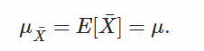
obviously(明顯) in practice, an infinite sample size is impossible). In other words, we can write (and we also checked this result

experimentally) that:

And if you don't care so much about the mathematics and just want to understand how this applies(應用) to you (and the field

of rendering) you can just see this as "your estimation becomes better as you keep taking samples (i.e. as n increases)".

Eventually you have so many samples, that your estimation and the value of what you are trying to estimate are very close to

each other and even the same in theory when you have an inifinity of these samples. That's really all it "means".

（當 取樣數接近無限的時候，）