概述

1. Although the final output of a renderer like pbrt is a two-dimensional grid of colored pixels, incident radiance is actually a continuous function defined over the film plane.The manner in which the discrete pixel values are computed from this continuous function can noticeably affect the quality of the final image generated by the renderer; if this process is not performed carefully, artifacts will be present.

Fortunately, a relatively small amount of additional computation to this end can substantially improve the quality of the rendered images.

（整個 Film Plane 上的 incident radiance 實際上是一個連續函式 ，但是Pixel是離散的，這些離散的Pixel其實是從incident radiance 連續函式中計算出來）

2. sampling theory—the theory of taking discrete sample values from functions defined over continuous domains and then using those samples to reconstruct new functions that are similar to the original

.Building on principles of sampling theory, the Samplers in this chapter select sample points on the image plane at which incident radiance will be computed

（取樣的理論就是，從一個連續函式A中進行取樣，得到一些取樣點，利用這些取樣點，重新構造出一個新的函式B，使得函式B 相似於 原來的函式A）

Sampling Theory

1. When thinking about digital images, it is important to differentiate between image pixels, which represent the value of a function at a particular sample location

, and display pixels, which are physical objects that emit light with some distribution.

（Pixel 表示的就是 取樣一個函式的某一個位置得到的函式值）

2.

Displays use the image pixel values to construct a new image function over the display surface.This function is defined at all points on the display, not just the infinitesimal points of the digital image’s pixels. This process of taking a collection of sample values and converting them back to a continuous function is called reconstruction.

（顯示器 使用所有 Pixel 值來為整個螢幕構建一個新的影象函式，這個新的影象函式不只是和Pixel有關，還是和整個螢幕的所有的點都有關，這個收集取樣值和把他們轉成一個連續函式的過程叫做 reconstruction）

3. 

In order to compute the discrete pixel values in the digital image, it is necessary to sample the original continuously defined image function. In pbrt, like most other ray-tracing renderers, the only way to get information about the image function is to sample it by tracing rays.

（為了計算圖片裡面的離散畫素值，需要去取樣 原始的連續的圖片函式，在pbrt中，或者其他的光線追蹤渲染器，去獲得圖片函式資訊的唯一方式就是 發射線去取樣）

4. 

While an image could be generated by just sampling the function precisely at the pixel positions, a better result can be obtained by taking more samples at different positions and incorporating this additional information about the image function into the final pixel values.

5. 

Indeed, for the best-quality result, the pixel values should be computed such that the reconstructed image on the display device is as close as possible to the original image of the scene on the virtual camera’s film plane.

（最好的圖片質量就是，用 Pixel 來 重構 的圖片 儘可能地接近  真實相機拍出來的 相片）

6. 

Because the sampling and reconstruction process involves approximation, it introduces error known as aliasing, which can manifest itself in many ways, including jagged edges or flickering in animations. These errors occur because the sampling process is not able to capture all of the information from the continuously defined image function.

（走樣主要是因為，取樣的過程中沒有 在連續的圖片函式中 獲得足夠的資訊）

7. 

Because the only information available about f comes from the sample values at the positions x‘, ˜ f is unlikely to match f perfectly since there is no information about f ’s behavior between the samples.

（上面演示的就是，在 原函式 進行取樣，利用取樣點 重構 一個新的函數出來）

8.

Fourier analysis can be used to evaluate the quality of the match between the reconstructed function and the original.

（簡單理解：傅立葉分析 是用來評估 重構函式和原函式 的差別大不大）

The Frequency Domain And The Fourier Transform

1. 

One of the foundations of Fourier analysis is the Fourier transform, which represents a function in the frequency domain. (We will say that functions are normally expressed in the spatial domain.) Consider the two functions graphed in Figure 7.2. The function in Figure 7.2(a) varies relatively slowly as a function of x, while the function in Figure 7.2(b) varies much more rapidly. The slower-varying function is said to have lower frequency content. Figure 7.3 shows the frequency space representations of these two functions;the lower-frequency function’s representation goes to zero more quickly than the higherfrequency function.

（Fourier transform  可以用 把一個 函式從 spatial domain 變到 frequency domain）

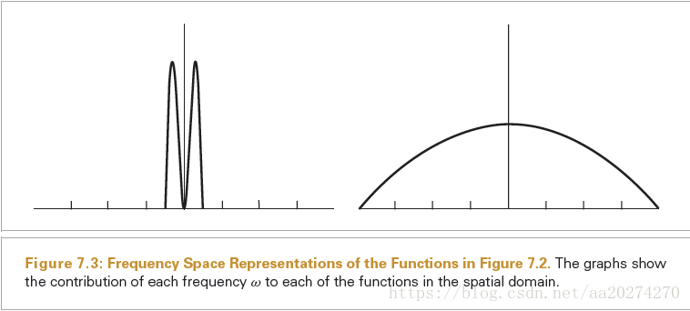
Most functions can be decomposed into a weighted sum of shifted sinusoids. This remarkable fact was first described by Joseph Fourier, and the Fourier transform converts a function into this representation. This frequency space representation of a function gives insight into some of its characteristics—the distribution of frequencies in the sine functions corresponds to the distribution of frequencies in the original function. Using this form, it is possible to use Fourier analysis to gain insight into the error that is introduced by the sampling and reconstruction process, and how to reduce the perceptual impact of this error.

（Fourier transform  可以用 把一個 函式從 spatial domain 變到 frequency domain，在 frequency domain 中表示一個函式的話，可以更方便地看清楚這個函式的 一些特徵，方便查錯和糾錯）

2. 

The Fourier transform of a one-dimensional function f (x) is

The new function F is a function of frequency, ω。

We will denote the Fourier transform operator by , such that {f (x)} = F(ω).

 is clearly a linear operator—that is, {af (x)} = a{f (x)} for any scalar a, and {f (x) + g(x)} ={f (x)} + {g(x)}.

3. 

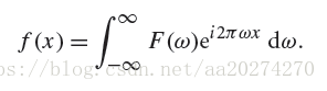
The inverse Fourier transform

Ideal Sampling And Reconstruction

1. （數學來表示取樣）

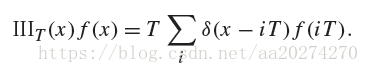
Recall that the sampling process requires us to choose a set of equally spaced sample positions and compute the function’s value at those positions. Formally, this corresponds to multiplying the function by a “shah,” or “impulse train,” function, an infinite sum of equally spaced delta functions. The shah  is defined as

where T defines the period, or sampling rate. This formal definition of sampling is illustrated in Figure 7.4. The multiplication yields an infinite sequence of values of the function at equally spaced points:

2. （重構函式）

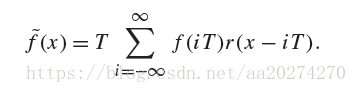
These sample values can be used to define a reconstructed function  by choosing a reconstruction filter function r(x) and computing the convolution

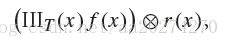
where the convolution operation ⊗ is defined as

For reconstruction, convolution gives a weighted sum of scaled instances of the reconstruction filter centered at the sample points:

For example, in Figure 7.1, the triangle reconstruction filter, f (x) = max(0, 1− |x|), was used. Figure 7.5 shows the scaled triangle functions used for that example.

We have gone through a process that may seem gratuitiously complex in order to end up at an intuitive result: the reconstructed function ~f(x) can be obtained by interpolating among the samples in some manner. By setting up this background carefully, however, Fourier analysis can now be applied to the process more easily.

We can gain a deeper understanding of the sampling process by analyzing the sampled function in the frequency domain.

In particular, we will be able to determine the conditions under which the original function can be exactly recovered from its values at the sample locations—a very powerful result. For the discussion here, we will assume for now that the function f (x) is band limited—there exists some frequency ω0 such that f (x) contains no frequencies greater than ω0. By definition, band-limited functions have frequency space representations with compact support, such that F(ω) = 0 for all |ω|>ω0.