
梯度下降方法實現邏輯迴歸效能
Logistic Regression
#三大件,%將那些用matplotlib繪製的圖顯示在頁面裡而不是彈出一個視窗
import numpy as np
import pandas as pd
import matplotlib.pyplot as plt
%matplotlib inline #由於 %matplotlib inline 的存在,當輸入plt.plot(x,y_1)後,不必再輸入 plt.show(),影象將自動顯示出來
#os.sep 可以取代作業系統特定的路徑分割符
import os
path = 'data' + os.sep + 'LogiReg_data.txt'
pdData = pd.read_csv(path, header=None, names=['Exam 1', 'Exam 2', 'Admitted'])
pdData.head()

positive = pdData[pdData['Admitted'] == 1]
negative = pdData[pdData['Admitted'] == 0]
fig, ax = plt.subplots(figsize=(10,5)) #固定搭配 fig, ax = plt.subplots(figsize=(12,8),ncols=2,nrows=1)#該方法會返回畫圖物件和座標物件ax,figsize是設定子圖長寬
ax.scatter(positive['Exam 1'], positive['Exam 2'], s=30, c='b', marker='o', label='Admitted')
ax.scatter(negative['Exam 1'], negative['Exam 2'], s=30, c='r', marker='x', label='Not Admitted')
ax.legend() #show
ax.set_xlabel('Exam 1 Score')
ax.set_ylabel('Exam 2 Score')

The logistic regression
目標:建立分類器(求解出三個引數 θ0θ1θ2θ0θ1θ2)
設定閾值,根據閾值判斷錄取結果
要完成的模組
sigmoid : 對映到概率的函式
model : 返回預測結果值
cost : 根據引數計算損失
gradient : 計算每個引數的梯度方向
descent : 進行引數更新
accuracy: 計算精度
sigmoid : 對映到概率的函式
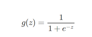
def sigmoid(z):
return 1 / (1 + np.exp(-z))
nums = np.arange(-10, 10, step=1) #creates a vector containing 20 equally spaced values from -10 to 10
fig, ax = plt.subplots(figsize=(12,4))
ax.plot(nums, sigmoid(nums), 'r') #x,y,color

np.dot()返回的是兩個陣列的點積(dot product)
1.如果處理的是一維陣列,則得到的是兩陣列的內積
In : d = np.arange(0,9)
Out: array([0, 1, 2, 3, 4, 5, 6, 7, 8])
In : e = d[::-1]
Out: array([8, 7, 6, 5, 4, 3, 2, 1, 0])

In : np.dot(d,e)
Out: 84
2.如果是二維陣列(矩陣)之間的運算,則得到的是矩陣積(mastrix product)
In : a = np.arange(1,5).reshape(2,2)
Out:
array([[1, 2],
[3, 4]])
In : b = np.arange(5,9).reshape(2,2)
Out: array([[5, 6],
[7, 8]])
In : np.dot(a,b)
Out:
array([[19, 22],
[43, 50]])
3. a.dot(b) 與 np.dot(a,b)效果相同
#預測函式模組
def model(X, theta):
return sigmoid(np.dot(X, theta.T))


y = 0,1代表類別
pdData.insert(0, 'Ones', 1) #第一列插入全為1的一列
# set X (training data) and y (target variable)
orig_data = pdData.as_matrix() # 返回不是Numpy矩陣,而是Numpy陣列。
cols = orig_data.shape[1]
X = orig_data[:,0:cols-1]
y = orig_data[:,cols-1:cols]
theta = np.zeros([1, 3]) #構造引數,進行佔位

def cost(X, y, theta):
left = np.multiply(-y, np.log(model(X, theta))) #等式左邊 這裡model(X, theta) == ![]()
right = np.multiply(1 - y, np.log(1 - model(X, theta)))
return np.sum(left - right) / (len(X))
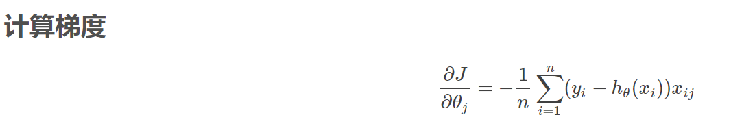
def gradient(X, y, theta):
grad = np.zeros(theta.shape) #theta數 = 求導次數,即解的數
error = (model(X, theta)- y).ravel() #yi---真實值,hx----預測值
for j in range(len(theta.ravel())): #for each parmeter
term = np.multiply(error, X[:,j])
grad[0, j] = np.sum(term) / len(X) #這裡X相當於樣本個數
return grad
numpy.ravel() 與numpy.flatten()
二者都是將多維陣列降位一維,
區別:
numpy.flatten()返回一份拷貝,對拷貝所做的修改不會影響(reflects)原始矩陣,
numpy.ravel()返回的是檢視(view,也頗有幾分C/C++引用reference的意味),會影響(reflects)原始矩陣。

Gradient descent
比較3種不同梯度下降方法
STOP_ITER = 0 #按次數
STOP_COST = 1 #損失
STOP_GRAD = 2 #梯度
def stopCriterion(type, value, threshold):
#設定三種不同的停止策略
if type == STOP_ITER: return value > threshold # threshold閾值
elif type == STOP_COST: return abs(value[-1]-value[-2]) < threshold
elif type == STOP_GRAD: return np.linalg.norm(value) < threshold
Python中fabs(x)方法返回x的絕對值。雖然類似於abs()函式,但是兩個函式之間存在以下差異:
-
abs()是一個內建函式,而fabs()在math模組中定義的。 -
fabs()函式只適用於float和integer型別,而abs()也適用於複數。
linalg=linear(線性)+algebra(代數),norm則表示範數。
函式引數
x_norm=np.linalg.norm(x, ord=None, axis=None, keepdims=False)
①x: 表示矩陣(也可以是一維)
②ord:範數型別
向量的範數:
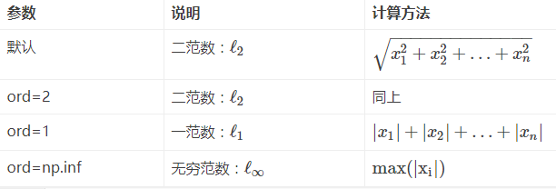
計算機領域 用的比較多的就是迭代過程中收斂性質的判斷,如果理解上述的意義,在計算機領域,一般迭代前後步驟的差值的範數表示其大小,常用的是二範數,差值越小表示越逼近實際值,可以認為達到要求的精度,收斂
import numpy.random
#洗牌 set X (trainning data) and y (target variable)
def shuffleData(data):
np.random.shuffle(data)
cols = data.shape[1]
X = data.iloc[:,0:cols-1] #x是所有行,去掉最後一列
y = data.iloc[:,cols-1:cols] #y是所有行,最後一列
return X, y
batch:批量----一次性拿多少個樣本去做
import time
def descent(data, theta, batchSize, stopType, thresh, alpha):
#梯度下降求解
init_time = time.time()
i = 0 # 迭代次數
k = 0 # batch:批量----一次性拿多少個樣本去做
X, y = shuffleData(data)
grad = np.zeros(theta.shape)
costs = [cost(X, y, theta)]
while True:
grad = gradient(X[k:k+batchSize], y[k:k+batchSize], theta)
k += batchSize #取batch數量個數據
if k >= n:
k = 0
X, y = shuffleData(data) #重新洗牌
theta = theta - alpha*grad # 引數更新
costs.append(cost(X, y, theta)) # 計算新的損失
i += 1
if stopType == STOP_ITER: value = i
elif stopType == STOP_COST: value = costs
elif stopType == STOP_GRAD: value = grad
if stopCriterion(stopType, value, thresh): break
return theta, i-1, costs, grad, time.time() - init_time
#此處的程式碼是將迭代的過程以圖表的形式展示
def runExpe(data, theta, batchSize, stopType, thresh, alpha):
#import pdb; pdb.set_trace(); 斷點除錯
pdb 是 python 自帶的一個包,為 python 程式提供了一種互動的原始碼除錯功能,主要特性包括設定斷點、單步除錯、進入函式除錯、檢視當前程式碼、檢視棧片段、動態改變變數的值等。
使用的時候要import pdb再用pdb.set_trace()設定一個斷點,執行程式的時候就會停在這。
theta, iter, costs, grad, dur = descent(data, theta, batchSize, stopType, thresh, alpha)
name = "Original" if (data[:,1]>2).sum() > 1 else "Scaled"
name += " data - learning rate: {} - ".format(alpha)
if batchSize==n: strDescType = "Gradient"
elif batchSize==1: strDescType = "Stochastic"
else: strDescType = "Mini-batch ({})".format(batchSize)
name += strDescType + " descent - Stop: "
if stopType == STOP_ITER: strStop = "{} iterations".format(thresh)
elif stopType == STOP_COST: strStop = "costs change < {}".format(thresh)
else: strStop = "gradient norm < {}".format(thresh)
name += strStop
print ("***{}\nTheta: {} - Iter: {} - Last cost: {:03.2f} - Duration: {:03.2f}s".format(
name, theta, iter, costs[-1], dur))
fig, ax = plt.subplots(figsize=(12,4))
ax.plot(np.arange(len(costs)), costs, 'r')
ax.set_xlabel('Iterations')
ax.set_ylabel('Cost')
ax.set_title(name.upper() + ' - Error vs. Iteration')
return theta