上一篇博文的內容整理了我們如何去近似價值函式或者是動作價值函式的方法： \[ V_{\theta}(s)\approx V^{\pi}(s) \\ Q_{\theta}(s)\approx Q^{\pi}(s, a) \] 通過機器學習的方法我們一旦近似了價值函式或者是動作價值函式就可以通過一些策略進行控制，比如 \(\epsilon\)-greedy。

那麼我們簡單回顧下 RL 的學習目標：通過 agent 與環境進行互動，獲取累計回報最大化。既然我們最終要學習如何與環境互動的策略，那麼我們可以直接學習策略嗎，而之前先近似價值函式，再通過貪婪策略控制的思路更像是"曲線救國"。 這就是本篇文章的內容，我們如何直接來學習策略，用數學的形式表達就是： \[\pi_{\theta}(s, a) = P[a | s, \theta]\]

這就是被稱為策略梯度（Policy Gradient，簡稱PG）演算法。

當然，本篇內容同樣的是針對 model-free 的強化學習。

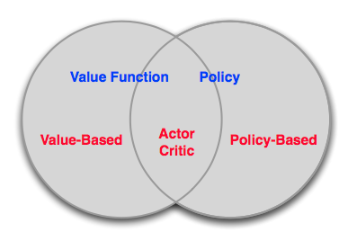
Value-Based vs. Policy-Based RL

Value-Based：

• 學習價值函式
• Implicit policy，比如 \(\epsilon\)-greedy

Policy-Based：

• 沒有價值函式
• 直接學習策略

Actor-Critic：

• 學習價值函式
• 學習策略

三者的關係可以形式化地表示如下：

認識到 Value-Based 與 Policy-Based 區別後，我們再來討論下 Policy-Based RL 的優缺點：

優點：

• 收斂性更好
• 對於具有高維或者連續動作空間的問題更加有效
• 可以學習隨機策略

缺點：

• 絕大多數情況下收斂到區域性最優點，而非全域性最優
• 評估一個策略一般情況下低效且存在較高的方差

Policy Search

我們首先定義下目標函式。

Policy Objective Functions

目標：給定一個帶有引數 \(\theta\) 的策略 \(\pi_{\theta}(s, a)\)，找到最優的引數 \(\theta\)。 但是我們如何評估不同引數下策略 \(\pi_{\theta}(s, a)\) 的優劣呢？

• 對於episode 任務來說，我們可以使用start value： \[J_1(\theta)=V^{\pi_{\theta}}(s_1)=E_{\pi_{\theta}}[v_1]\]
• 對於連續性任務來說，我們可以使用 average value： \[J_{avV}(\theta)=\sum_{s}d^{\pi_{\theta}}(s)V^{\pi_{\theta}}(s)\] 或者每一步的平均回報： \[J_{avR}(\theta)=\sum_{s}d^{\pi_{\theta}}(s)\sum_{a}\pi_{\theta}(s, a)R_s^a\] 其中 \(d^{\pi_{\theta}}(s)\) 是馬爾卡夫鏈在 \(\pi_{\theta}\) 下的靜態分佈。

Policy Optimisation

在明確目標以後，我們再來看基於策略的 RL 為一個典型的優化問題：找出 \(\theta\) 最大化 \(J(\theta)\)。 最優化的方法有很多，比如不依賴梯度（gradient-free）的演算法：

• 爬山演算法
• 模擬退火
• 進化演算法
• ...

但是一般來說，如果我們能在問題中獲得梯度的話，基於梯度的最優化方法具有比較好的效果：

• 梯度下降
• 共軛梯度
• 擬牛頓法
• ...

我們本篇討論梯度下降的方法。

策略梯度定理

假設策略 \(\pi_{\theta}\) 為零的時候可微，並且已知梯度 \(\triangledown_{\theta}\pi_{\theta}(s, a)\)，定義 \(\triangledown_{\theta}\log\pi_{\theta}(s, a)\) 為得分函式（score function）。二者關係如下： \[\triangledown_{\theta}\pi_{\theta}(s, a) = \triangledown_{\theta}\pi_{\theta}(s, a) \frac{\triangledown_{\theta}\pi_{\theta}(s, a)}{\pi_{\theta}(s, a)}=\pi_{\theta}(s, a)\triangledown_{\theta}\log\pi_{\theta}(s, a)\] 接下來我們考慮一個只走一步的MDP，對它使用策略梯度下降。\(\pi_{\theta}(s, a)\) 表示關於引數 \(\theta\) 的函式，對映是 \(p(a|s,\theta)\)。它在狀態 \(s\) 向前走一步，獲得獎勵\(r=R_{s, a}\)。那麼選擇行動 \(a\) 的獎勵為 \(\pi_{\theta}(s, a)R_{s, a}\)，在狀態 \(s\) 的加權獎勵為 \(\sum_{a\in A}\pi_{\theta}(s, a)R_{s, a}\)，應用策略所能獲得的獎勵期望及梯度為： \[ J(\theta)=E_{\pi_{\theta}}[r] = \sum_{s\in S}d(s)\sum_{a\in A}\pi_{\theta}(s, a)R_{s, a}\\ \triangledown_{\theta}J(\theta) = \color{Red}{\sum_{s\in S}d(s)\sum_{a\in A}\pi_{\theta}(s, a)}\triangledown_{\theta}\log\pi_{\theta}(s, a)R_{s, a}=E_{\pi_{\theta}}[\triangledown_{\theta}\log\pi_{\theta}(s, a)r] \]

再考慮走了多步的MDP，使用 \(Q^{\pi_{\theta}}(s, a)\) 代替獎勵值 \(r\)，對於任意可微的策略，策略梯度為： \[\triangledown_{\theta}J(\theta) = E_{\pi_{\theta}}[\triangledown_{\theta}\log\pi_{\theta}(s, a)Q^{\pi_{\theta}}(s, a)]\]

策略梯度定理

對於任意可微策略 \(\pi_{\theta}(s, a)\)，任意策略目標方程 \(J = J_1, J_{avR}, ...\)，策略梯度： \[\triangledown_{\theta}J(\theta) = E_{\pi_{\theta}}[\triangledown_{\theta}\log\pi_{\theta}(s, a)Q^{\pi_{\theta}}(s, a)]\]

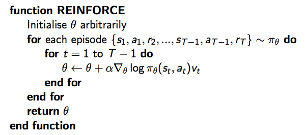
蒙特卡洛策略梯度演算法（REINFORCE）

Monte-Carlo策略梯度演算法，即REINFORCE：

• 通過取樣episode來更新引數：；
• 使用隨機梯度上升法更新引數；
• 使用return \(v_t\) 作為 \(Q^{\pi_{\theta}}(s_t, a_t)\) 的無偏估計

則 \(\Delta\theta_t = \alpha \triangledown_{\theta}\log\pi_{\theta}(s_t, a_t)v_t\)，具體如下：

Actir-Critic 策略梯度演算法

Monte-Carlo策略梯度的方差較高，因此放棄用return來估計行動-價值函式Q，而是使用 critic 來估計Q： \[Q_w(s, a)\approx Q^{\pi_{\theta}}(s, a)\] 這就是大名鼎鼎的 Actor-Critic 演算法，它有兩套引數：

• Critic：更新動作價值函式引數 \(w\)
• Actor： 朝著 Critic 方向更新策略引數 \(\theta\)

Actor-Critic 演算法是一個近似的策略梯度演算法： \[ \triangledown_\theta J(\theta)\approx E_{\pi_{\theta}}[\triangledown_{\theta}\log \pi_{\theta}(s, a)Q_w(s, a)]\\ \Delta\theta = \alpha\triangledown_\theta\log\pi_{\theta}(s,a)Q_w(s,a) \]

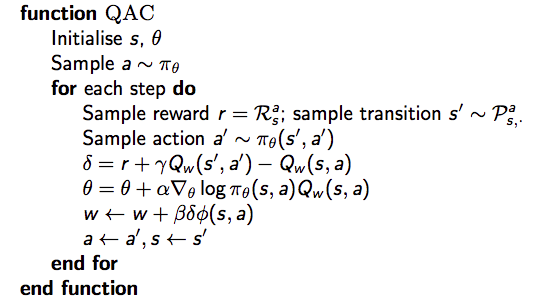
Critic 本質就是在進行策略評估：How good is policy \(\pi_{\theta}\) for current parameters \(\theta\). 策略評估我們之前介紹過MC、TD、TD(\(\lambda\))，以及價值函式近似方法。如下所示，簡單的 Actir-Critic 演算法 Critic 為動作價值函式近似，使用最為簡單的線性方程，即：\(Q_w(s, a) = \phi(s, a)^T w\)，具體的虛擬碼如下所示：

在 Actir-Critic 演算法中，對策略進行了估計，這會產生誤差（bias），但是當滿足以下兩個條件時，策略梯度是準確的：

• 價值函式的估計值沒有和策略相違背，即：\(\triangledown_w Q_w(s,a) = \triangledown_\theta\log\pi_{\theta}(s,a)\)
• 價值函式的引數w能夠最小化誤差，即：\(\epsilon = E_{\pi_{\theta}}[(Q^{\pi_{\theta}}(s, a) - Q_w(s,a))^2]\)

優勢函式

另外，我們可以通過將策略梯度減去一個基線函式（baseline funtion）B(s)，可以在不改變期望的情況下降低方差（variance）。證明不改變期望，就是證明相加和為0： \[ \begin{align} E_{\pi_{\theta}}[\triangledown_\theta\log\pi_{\theta}(s,a)B(s)] &=\sum_{s\in S}d^{\pi_{\theta}}(s)\sum_a \triangledown_\theta\pi_{\theta}(s, a)B(s)\\ &=\sum_{s\in S}d^{\pi_{\theta}}(s)B(s)\triangledown_\theta\sum_{a\in A}\pi_{\theta}(s,a )\\ &= 0 \end{align} \]

狀態價值函式 \(V^{\pi_{\theta}}(s)\) 是一個好的基線。因此可以通過使用優勢函式（Advantage function）\(A^{\pi_{\theta}}(s,a)\) 來重寫價值梯度函式。 \[ A^{\pi_{\theta}}(s,a)=Q^{\pi_{\theta}}(s,a)-V^{\pi_{\theta}}(s)\\ \triangledown_\theta J(\theta)=E_{\pi_{\theta}}[\triangledown_\theta\log\pi_{\theta}(s,a)A^{\pi_{\theta}}(s,a)] \]

設 \(V^{\pi_{\theta}}(s)\) 是真實的價值函式，TD演算法利用bellman方程來逼近真實值，誤差為 \(\delta^{\pi_{\theta}}=r+\gamma V^{\pi_{\theta}}(s') - V^{\pi_{\theta}}(s)\)。該誤差是優勢函式的無偏估計。因此我們可以使用該誤差計算策略梯度： \[\triangledown_\theta J(\theta)=E_{\pi_{\theta}}[\triangledown_\theta\log\pi_{\theta}(s,a)\delta^{\pi_{\theta}}]\] 該方法只需要critic，不需要actor。更多關於 Advantage Function 的可以看這裡。

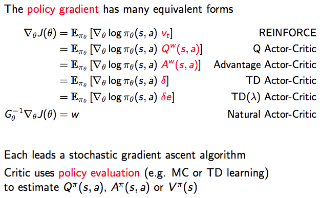
最後總結一下策略梯度演算法：

Reference