[Keras深度學習淺嘗]實戰四· Embedding實現 IMDB資料集影評文字分類
阿新 • • 發佈:2018-12-22
[Keras深度學習淺嘗]實戰四· Embedding實現 IMDB資料集影評文字分類
此實戰來源於TensorFlow Keras官方教程
先更新程式碼在這裡,後面找時間理解註釋一下。
# TensorFlow and tf.keras
import os
os.environ["KMP_DUPLICATE_LIB_OK"]="TRUE"
import tensorflow as tf
from tensorflow import keras
# Helper libraries
import numpy as np
import matplotlib.pyplot as 1.12.0
imdb = keras.datasets.imdb

(train_data, train_labels), (test_data, test_labels) = imdb.load_data(num_words=10000)
Downloading data from https://storage.googleapis.com/tensorflow/tf-keras-datasets/imdb.npz
17465344/17464789 [==============================] - 12s 1us/step
print("Training entries: {}, labels: {}".format(len(train_data), len(train_labels)))
Training entries: 25000, labels: 25000
print(train_data[0])
len(train_data[0]), len(train_data[1])
[1, 14, 22, 16, 43, 530, 973, 1622, 1385, 65, 458, 4468, 66, 3941, 4, 173, 36, 256, 5, 25, 100, 43, 838, 112, 50, 670, 2, 9, 35, 480, 284, 5, 150, 4, 172, 112, 167, 2, 336, 385, 39, 4, 172, 4536, 1111, 17, 546, 38, 13, 447, 4, 192, 50, 16, 6, 147, 2025, 19, 14, 22, 4, 1920, 4613, 469, 4, 22, 71, 87, 12, 16, 43, 530, 38, 76, 15, 13, 1247, 4, 22, 17, 515, 17, 12, 16, 626, 18, 2, 5, 62, 386, 12, 8, 316, 8, 106, 5, 4, 2223, 5244, 16, 480, 66, 3785, 33, 4, 130, 12, 16, 38, 619, 5, 25, 124, 51, 36, 135, 48, 25, 1415, 33, 6, 22, 12, 215, 28, 77, 52, 5, 14, 407, 16, 82, 2, 8, 4, 107, 117, 5952, 15, 256, 4, 2, 7, 3766, 5, 723, 36, 71, 43, 530, 476, 26, 400, 317, 46, 7, 4, 2, 1029, 13, 104, 88, 4, 381, 15, 297, 98, 32, 2071, 56, 26, 141, 6, 194, 7486, 18, 4, 226, 22, 21, 134, 476, 26, 480, 5, 144, 30, 5535, 18, 51, 36, 28, 224, 92, 25, 104, 4, 226, 65, 16, 38, 1334, 88, 12, 16, 283, 5, 16, 4472, 113, 103, 32, 15, 16, 5345, 19, 178, 32]


(218, 189)
# A dictionary mapping words to an integer index
word_index = imdb.get_word_index()

# The first indices are reserved
word_index = {k:(v+3) for k,v in word_index.items()}
word_index["<PAD>"] = 0
word_index["<START>"] = 1
word_index["<UNK>"] = 2  # unknown
word_index["<UNUSED>"] = 3

reverse_word_index = dict([(value, key) for (key, value) in word_index.items()])

def decode_review(text):
    return ' '.join([reverse_word_index.get(i, '?') for i in text])
Downloading data from https://storage.googleapis.com/tensorflow/tf-keras-datasets/imdb_word_index.json
1646592/1641221 [==============================] - 2s 1us/step
decode_review(train_data[0])
"<START> this film was just brilliant casting location scenery story direction everyone's really suited the part they played and you could just imagine being there robert <UNK> is an amazing actor and now the same being director <UNK> father came from the same scottish island as myself so i loved the fact there was a real connection with this film the witty remarks throughout the film were great it was just brilliant so much that i bought the film as soon as it was released for <UNK> and would recommend it to everyone to watch and the fly fishing was amazing really cried at the end it was so sad and you know what they say if you cry at a film it must have been good and this definitely was also <UNK> to the two little boy's that played the <UNK> of norman and paul they were just brilliant children are often left out of the <UNK> list i think because the stars that play them all grown up are such a big profile for the whole film but these children are amazing and should be praised for what they have done don't you think the whole story was so lovely because it was true and was someone's life after all that was shared with us all"
train_data = keras.preprocessing.sequence.pad_sequences(train_data,
                                                        value=word_index["<PAD>"],
                                                        padding='post',
                                                        maxlen=256)

test_data = keras.preprocessing.sequence.pad_sequences(test_data,
                                                       value=word_index["<PAD>"],
                                                       padding='post',
                                                       maxlen=256)
len(train_data[0]), len(train_data[1])
(256, 256)
print(train_data[0])
[   1   14   22   16   43  530  973 1622 1385   65  458 4468   66 3941
    4  173   36  256    5   25  100   43  838  112   50  670    2    9
   35  480  284    5  150    4  172  112  167    2  336  385   39    4
  172 4536 1111   17  546   38   13  447    4  192   50   16    6  147
 2025   19   14   22    4 1920 4613  469    4   22   71   87   12   16
   43  530   38   76   15   13 1247    4   22   17  515   17   12   16
  626   18    2    5   62  386   12    8  316    8  106    5    4 2223
 5244   16  480   66 3785   33    4  130   12   16   38  619    5   25
  124   51   36  135   48   25 1415   33    6   22   12  215   28   77
   52    5   14  407   16   82    2    8    4  107  117 5952   15  256
    4    2    7 3766    5  723   36   71   43  530  476   26  400  317
   46    7    4    2 1029   13  104   88    4  381   15  297   98   32
 2071   56   26  141    6  194 7486   18    4  226   22   21  134  476
   26  480    5  144   30 5535   18   51   36   28  224   92   25  104
    4  226   65   16   38 1334   88   12   16  283    5   16 4472  113
  103   32   15   16 5345   19  178   32    0    0    0    0    0    0
    0    0    0    0    0    0    0    0    0    0    0    0    0    0
    0    0    0    0    0    0    0    0    0    0    0    0    0    0
    0    0    0    0]
網路模型的介紹:
1,輸入網路的形狀為(-1,256)
2,Embedding後為(-1,256,16)網路引數為(10000,16)
3,GlobalAveragePooling1D後為(-1,16)詳細介紹見此
4,Dense1後(-1,16)網路引數為w:1616 + b:116 共計272
4,Dense2後(-1,1)網路引數為w:161 + b:11 共計17個引數
vocab_size = 10000

model = keras.Sequential()
model.add(keras.layers.Embedding(vocab_size, 16))
model.add(keras.layers.GlobalAveragePooling1D())
model.add(keras.layers.Dense(16, activation=tf.nn.relu))
model.add(keras.layers.Dense(1, activation=tf.nn.sigmoid))

model.summary()
_________________________________________________________________
Layer (type)                 Output Shape              Param #
=================================================================
embedding (Embedding)        (None, None, 16)          160000
_________________________________________________________________
global_average_pooling1d (Gl (None, 16)                0
_________________________________________________________________
dense (Dense)                (None, 16)                272
_________________________________________________________________
dense_1 (Dense)              (None, 1)                 17
=================================================================
Total params: 160,289
Trainable params: 160,289
Non-trainable params: 0
_________________________________________________________________
model.compile(optimizer=tf.train.AdamOptimizer(),
              loss='binary_crossentropy',
              metrics=['accuracy'])
x_val = train_data[:10000]
partial_x_train = train_data[10000:]

y_val = train_labels[:10000]
partial_y_train = train_labels[10000:]
history = model.fit(partial_x_train,
                    partial_y_train,
                    epochs=20,
                    batch_size=512,
                    validation_data=(x_val, y_val),
                    verbose=1)
Train on 15000 samples, validate on 10000 samples
Epoch 1/20
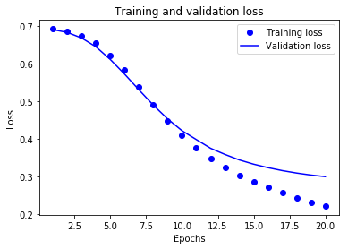
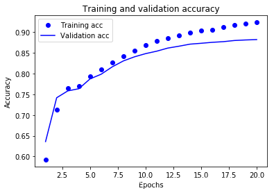
15000/15000 [==============================] - 3s 215us/step - loss: 0.6919 - acc: 0.5925 - val_loss: 0.6899 - val_acc: 0.6360
Epoch 2/20
15000/15000 [==============================] - 2s 159us/step - loss: 0.6863 - acc: 0.7131 - val_loss: 0.6824 - val_acc: 0.7418
Epoch 3/20
15000/15000 [==============================] - 2s 155us/step - loss: 0.6746 - acc: 0.7652 - val_loss: 0.6676 - val_acc: 0.7583
Epoch 4/20
15000/15000 [==============================] - 2s 153us/step - loss: 0.6534 - acc: 0.7707 - val_loss: 0.6440 - val_acc: 0.7636
Epoch 5/20
15000/15000 [==============================] - 2s 153us/step - loss: 0.6221 - acc: 0.7933 - val_loss: 0.6104 - val_acc: 0.7872
Epoch 6/20
15000/15000 [==============================] - 2s 153us/step - loss: 0.5820 - acc: 0.8095 - val_loss: 0.5713 - val_acc: 0.7985
Epoch 7/20
15000/15000 [==============================] - 2s 154us/step - loss: 0.5368 - acc: 0.8271 - val_loss: 0.5297 - val_acc: 0.8163
Epoch 8/20
15000/15000 [==============================] - 2s 159us/step - loss: 0.4907 - acc: 0.8427 - val_loss: 0.4891 - val_acc: 0.8306
Epoch 9/20
15000/15000 [==============================] - 3s 170us/step - loss: 0.4478 - acc: 0.8557 - val_loss: 0.4525 - val_acc: 0.8405
Epoch 10/20
15000/15000 [==============================] - 2s 165us/step - loss: 0.4089 - acc: 0.8692 - val_loss: 0.4213 - val_acc: 0.8482
Epoch 11/20
15000/15000 [==============================] - 2s 156us/step - loss: 0.3760 - acc: 0.8791 - val_loss: 0.3977 - val_acc: 0.8541
Epoch 12/20
15000/15000 [==============================] - 2s 153us/step - loss: 0.3483 - acc: 0.8852 - val_loss: 0.3745 - val_acc: 0.8616
Epoch 13/20
15000/15000 [==============================] - 3s 171us/step - loss: 0.3236 - acc: 0.8929 - val_loss: 0.3581 - val_acc: 0.8661
Epoch 14/20
15000/15000 [==============================] - 3s 171us/step - loss: 0.3031 - acc: 0.8981 - val_loss: 0.3436 - val_acc: 0.8711
Epoch 15/20
15000/15000 [==============================] - 3s 178us/step - loss: 0.2854 - acc: 0.9033 - val_loss: 0.3322 - val_acc: 0.8732
Epoch 16/20
15000/15000 [==============================] - 3s 173us/step - loss: 0.2702 - acc: 0.9057 - val_loss: 0.3230 - val_acc: 0.8755
Epoch 17/20
15000/15000 [==============================] - 2s 165us/step - loss: 0.2557 - acc: 0.9131 - val_loss: 0.3152 - val_acc: 0.8771
Epoch 18/20
15000/15000 [==============================] - 2s 155us/step - loss: 0.2431 - acc: 0.9171 - val_loss: 0.3087 - val_acc: 0.8799
Epoch 19/20
15000/15000 [==============================] - 2s 155us/step - loss: 0.2315 - acc: 0.9213 - val_loss: 0.3033 - val_acc: 0.8812
Epoch 20/20
15000/15000 [==============================] - 2s 164us/step - loss: 0.2213 - acc: 0.9236 - val_loss: 0.2991 - val_acc: 0.8821
results = model.evaluate(test_data, test_labels)

print(results)
25000/25000 [==============================] - 1s 38us/step
[0.3124048164367676, 0.87232]
history_dict = history.history
history_dict.keys()
dict_keys(['val_loss', 'val_acc', 'loss', 'acc'])
import matplotlib.pyplot as plt

acc = history.history['acc']
val_acc = history.history['val_acc']
loss = history.history['loss']
val_loss = history.history['val_loss']

epochs = range(1, len(acc) + 1)

# "bo" is for "blue dot"
plt.plot(epochs, loss, 'bo', label='Training loss')
# b is for "solid blue line"
plt.plot(epochs, val_loss, 'b', label='Validation loss')
plt.title('Training and validation loss')
plt.xlabel('Epochs')
plt.ylabel('Loss')
plt.legend()

plt.show()

plt.clf()   # clear figure
acc_values = history_dict['acc']
val_acc_values = history_dict['val_acc']

plt.plot(epochs, acc, 'bo', label='Training acc')
plt.plot(epochs, val_acc, 'b', label='Validation acc')
plt.title('Training and validation accuracy')
plt.xlabel('Epochs')
plt.ylabel('Accuracy')
plt.legend()

plt.show()

