Linear Regression on Boston Housing Dataset

In my previous blog, I covered the basics of linear regression and gradient descent. To get hands-on linear regression we will take an original dataset and apply the concepts that we have learned.

We will take the Housing dataset which contains information about different houses in Boston. This data was originally a part of UCI Machine Learning Repository and has been removed now. We can also access this data from the scikit-learn library. There are 506 samples and 13 feature variables in this dataset. The objective is to predict the value of prices of the house using the given features.

So let’s get started.

First, we will import the required libraries.

Next, we will load the housing data from the scikit-learn library and understand it.

We print the value of the boston_dataset to understand what it contains. print(boston_dataset.keys()) gives

dict_keys(['data', 'target', 'feature_names', 'DESCR'])

• data: contains the information for various houses
• target: prices of the house
• feature_names: names of the features
• DESCR: describes the dataset

To know more about the features use boston_dataset.DESCR The description of all the features is given below:

CRIM: Per capita crime rate by townZN: Proportion of residential land zoned for lots over 25,000 sq. ftINDUS
 
: Proportion of non-retail business acres per townCHAS: Charles River dummy variable (= 1 if tract bounds river; 0 otherwise)NOX: Nitric oxide concentration (parts per 10 million)RM: Average number of rooms per dwellingAGE: Proportion of owner-occupied units built prior to 1940DIS: Weighted distances to five Boston employment centersRAD: Index of accessibility to radial highwaysTAX: Full-value property tax rate per $10,000PTRATIO: Pupil-teacher ratio by townB: 1000(Bk — 0.63)², where Bk is the proportion of [people of African American descent] by townLSTAT: Percentage of lower status of the populationMEDV: Median value of owner-occupied homes in $1000s

The prices of the house indicated by the variable MEDV is our target variable and the remaining are the feature variables based on which we will predict the value of a house.

We will now load the data into a pandas dataframe using pd.DataFrame. We then print the first 5 rows of the data using head()

We can see that the target value MEDV is missing from the data. We create a new column of target values and add it to the dataframe.

Data preprocessing

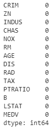
After loading the data, it’s a good practice to see if there are any missing values in the data. We count the number of missing values for each feature using isnull()

However, there are no missing values in this dataset as shown below.

Exploratory Data Analysis

Exploratory Data Analysis is a very important step before training the model. In this section, we will use some visualizations to understand the relationship of the target variable with other features.

Let’s first plot the distribution of the target variable MEDV. We will use the distplot function from the seaborn library.

We see that the values of MEDV are distributed normally with few outliers.

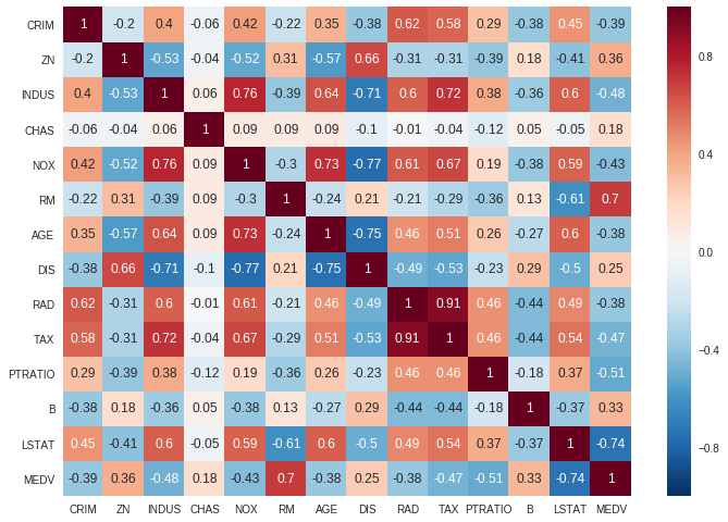
Next, we create a correlation matrix that measures the linear relationships between the variables. The correlation matrix can be formed by using the corr function from the pandas dataframe library. We will use the heatmap function from the seaborn library to plot the correlation matrix.

The correlation coefficient ranges from -1 to 1. If the value is close to 1, it means that there is a strong positive correlation between the two variables. When it is close to -1, the variables have a strong negative correlation.

Observations:

• To fit a linear regression model, we select those features which have a high correlation with our target variable MEDV. By looking at the correlation matrix we can see that RM has a strong positive correlation with MEDV (0.7) where as LSTAT has a high negative correlation with MEDV(-0.74).
• An important point in selecting features for a linear regression model is to check for multi-co-linearity. The features RAD, TAX have a correlation of 0.91. These feature pairs are strongly correlated to each other. We should not select both these features together for training the model. Check this for an explanation. Same goes for the features DIS and AGE which have a correlation of -0.75.

Based on the above observations we will RM and LSTAT as our features. Using a scatter plot let’s see how these features vary with MEDV.

Observations:

• The prices increase as the value of RM increases linearly. There are few outliers and the data seems to be capped at 50.
• The prices tend to decrease with an increase in LSTAT. Though it doesn’t look to be following exactly a linear line.

Preparing the data for training the model

We concatenate the LSTAT and RM columns using np.c_ provided by the numpy library.

Splitting the data into training and testing sets

Next, we split the data into training and testing sets. We train the model with 80% of the samples and test with the remaining 20%. We do this to assess the model’s performance on unseen data. To split the data we use train_test_split function provided by scikit-learn library. We finally print the sizes of our training and test set to verify if the splitting has occurred properly.

(404, 2) (102, 2)(404,)(102,)

Training and testing the model

We use scikit-learn’s LinearRegression to train our model on both the training and test sets.

Model evaluation

We will evaluate our model using RMSE and R2-score.

The model performance for training set -------------------------------------- RMSE is 5.6371293350711955 R2 score is 0.6300745149331701   

The model performance for testing set -------------------------------------- RMSE is 5.137400784702911R2 score is 0.6628996975186952

This is good to start with. In the upcoming blogs, we will look at ways to increase the model’s performance.

The complete Jupyter Notebook can be found here.

Conclusion

In this story, we applied the concepts of linear regression on the Boston housing dataset. I would recommend to try out other datasets as well.

Here are a few places you can look for data

Thanks for Reading!!

In the next part of this series, we will cover Polynomial Regression. Do watch this space for more.