Analyzing time series data in Pandas

In my previous tutorials, we have considered data preparation and visualization tools such as Numpy, Pandas, Matplotlib and Seaborn. In this tutorial, we are going to learn about Time Series, why it’s important, situations we will need to apply Time Series, and more specifically, we will learn how to analyze Time Series data using Pandas.

What is Time Series

Time Series is a set of data points or observations taken at specified times usually at equal intervals (e.g hourly, daily, weekly, quarterly, yearly, etc). Time Series is usually used to predict future occurrences based on previous observed occurrence or values. Predicting what would happen in the stock market tomorrow, volume of goods that would be sold in the coming week, whether or not price of an item would skyrocket in December, number of Uber rides over a period of time, etc; are some of the things we can do with Time Series Analysis.

Why we need Time series

Time series helps us understand past trends so we can forecast and plan for the future. For example, you own a coffee shop, what you’d likely see is how many coffee you sell every day or month and when you want to see how your shop has performed over the past six months, you’re likely going to add all the six month sales. Now, what if you want to be able to forecast sales for the next six months or year. In this kind of scenario, the only variable known to you is time (either in seconds, minutes, days, months, years, etc) — hence you need Time Series Analysis to predict the other unknown variables like trends, seasonality, etc.

Hence, it is important to note that in Time Series Analysis, the only known variable is — Time.

Why pandas makes it easy to work with Time Series

Pandas has proven very successful as a tool for working with Time Series data. This is because Pandas has some in-built datetime functions which makes it easy to work with a Time Series Analysis, and since time is the most important variable we work with here, it makes Pandas a very suitable tool to perform such analysis.

Components of Time Series

Generally, including those outside of the financial world, Time Series often contain the following features:

1. Trends: This refers to the movement of a series to relatively higher or lower values over a long period of time. For example, when the Time Series Analysis shows a pattern that is upward, we call it an Uptrend, and when the pattern is downward, we call it a Down trend, and if there was no trend at all, we call it a horizontal or stationary trend. One key thing to note is that trend usually happens for sometime and then disappears.
2. Seasonality: This refers to is a repeating pattern within a fixed time period. Although these patterns can also swing upward or downward, however, this is quite different from that of a trend because trend happens for a period of time and then disappears. However Seasonality keeps happening within a fixed time period. For example, when it’s Christmas, you discover more candies and chocolates are sold and this keeps happening every year.
3. Irregularity: This is also called noise. Irregularity happens for a short duration and it’s non depleting. A very good example is the case of Ebola. During that period, there was a massive demand for hand sanitizers which happened erratically/systematically in a way no one could have predicted, hence one could not tell how much number of sales could have been made or tell the next time there’s going to be another outbreak.
4. Cyclic: This is when a series is repeating upward and downward movement. It usually does not have a fixed pattern. It could happen in 6months, then two years later, then 4 years, then 1 year later. These kinds of patterns are much harder to predict.

When not to apply TS

Remember how we stated that the main variable here is Time? Same way, it is important to mention that we cannot apply Time Series analysis to a dataset when:

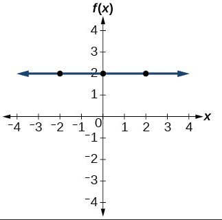
1. The variables/values are constant. For example, 5000 boxes of candies where sold last Christmas, and the Christmas before that. Since both values are the same, we cannot apply time series to predict sales for this year’s Christmas.

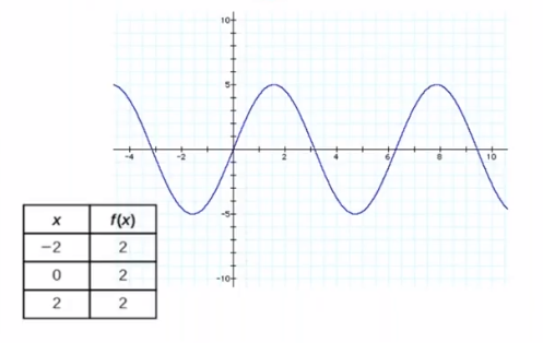
2. Values in the form of functions: There’s no point applying Time Series Analysis to a dataset when you can calculate values by simply using a formula or function.

Now that we have basic understanding of what Time Series is, let’s go ahead and work on an example to fully grasp how we can analyze a Time Series Data.

Forecasting the future of an Air Travel Company

In this example, we are asked to build a model to forecast the demand for flight tickets of a particular airline. We will be using the International Airline Passengers dataset . You can also download it from kaggle here.

Importing Packages and Data

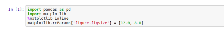
To begin, first thing we need to do is to import the packages we will use to perform our analysis: in this case, we’ll make use of pandas, to prepare our data and access the datetime functions and matplotlib to create our visualizations:

Now, let’s read our dataset to see what kind of data we have. As we see, the dataset has been classified into two columns; Month and Passengers traveling per month.

I usually like getting a summary of the dataset in case there’s a row with an empty value. Let’s go ahead and check by doing this:

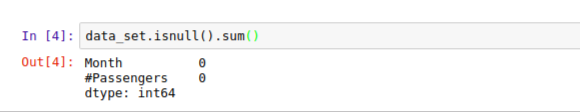
As we can see, we do not have any empty value in our dataset, so we’re free to continue our analysis. Now, what we will do is to confirm that the Month column is in datetime format and not string. Pandas .dtypes function makes this possible:

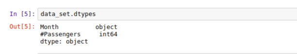
We can see that Month column is of a generic object type which could be a string. Since we want to perform time related actions on this data, we need to convert it to a datetime format before it can be useful to us. Let’s go ahead and do this using to_datetime() helper function, let’s cast the Month column to a datetime object instead of a generic object:

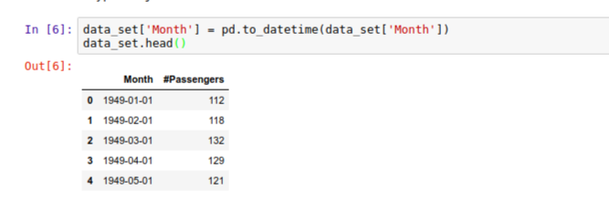
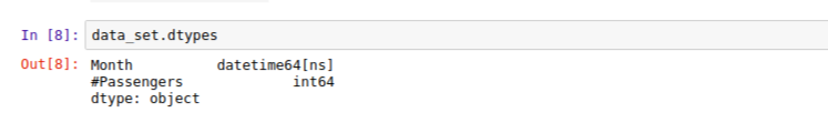
Notice how we now have date field generated for us as part of the Month column. By default, the date field assumes the first day of the month to fill in the values of the days that were not supplied. Now, if we go back and confirm the type, we can see that it’s now of type datetime :

Now, we need to set the datetime object as the index of the dataframe to allow us really explore our data. Let’s do this using the .set_index() method:

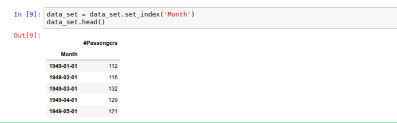
We can see now that the Month column is the index of our dataframe. Let’s go ahead and create our plot to see what our data looks like:

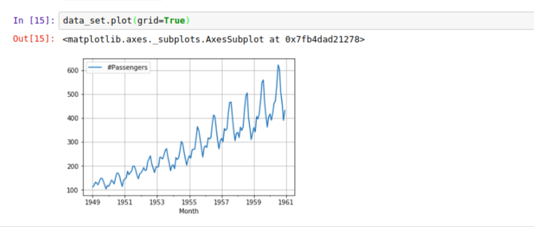
Note that in Time Series plots, time is usually plotted on the x-axis while the y-axis is usually the magnitude of the data.

Notice how the Month column was used as our x-axis and because we had previously casted our Month column to datetime, the year was specifically used to plot the graph.

By now, you should notice an upward trend indicating that the airline would have more passenger over time. Although there are ups and downs at every point in time, generally we can observe that the trend increases. Also we can notice how the ups and downs seem to be a bit regular, it means we might be observing a seasonal pattern here too. Let’s take a closer look by observing some year’s data:

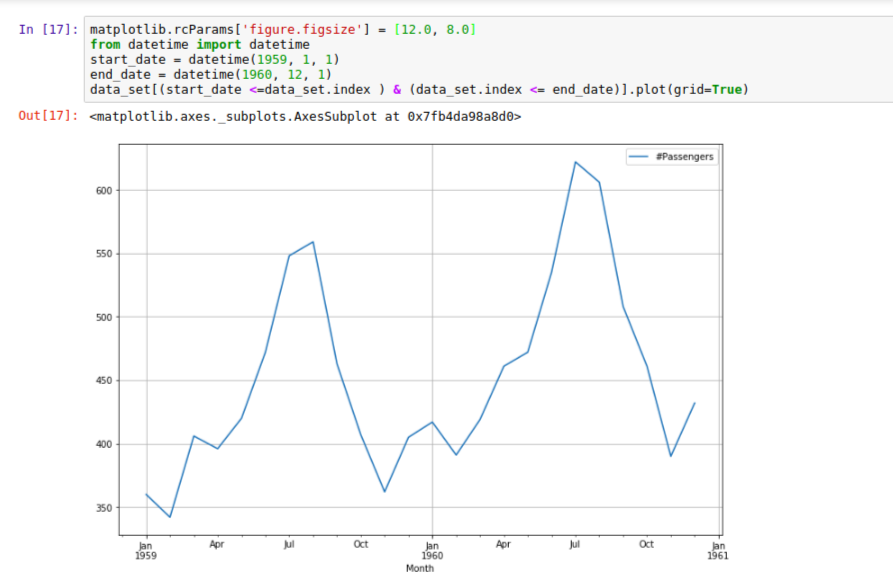
As we can see in the plot, there’s usually a spike between July and September which begins to drop by October, which implies that more people travel between July and September and probably travel less from October.

Remember we mentioned that there’s an upward trend and a seasonal pattern in our observation? There are usually a number of components [Scroll up to see explanation of Time Series components] in most Time Series analysis. Hence, what we need to do now is use Decomposition techniques to to deconstruct our observation into several components, each representing one of the underlying categories of patterns.

Decomposition of Time Series

There are a couple of models to consider during the Decomposition of Time Series data.1. Additive Model: This model is used when the variations around the trend does not vary with the level of the time series. Here the components of a time series are simply added together using the formula: y(t) = Level(t) + Trend(t) + Seasonality(t) + Noise(t)2. Multiplicative Model: Is used if the trend is proportional to the level of the time series. Here the components of a time series are simply multiplied together using the formula: y(t) = Level(t) * Trend(t) * Seasonality(t) *Noise(t)

For the sake of this tutorial, we will use the additive model because it is quick to develop, fast to train, and provide interpretable patterns. We also need to import which has a tsa (time series analysis) package as well as the seasonal_decompose() function we need:

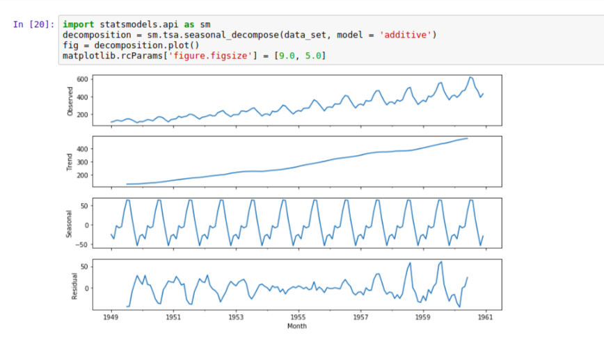
Now we have a much clearer plot showing us that the trend is going up, and the seasonality following a regular pattern.

One last thing we will do is plot the trend alongside the observed time series. To do this, we will use Matplotlib’s .YearLocator() function to set each year to begin from the month of January month=1 , and month as the minor locator showing ticks for every 3 months (intervals=3). Then we plot our dataset (and gave it blue color) using the index of the dataframe as x-axis and the number of Passengers for the y-axis.We did the same for the trend observations which we plotted in red color.

import matplotlib.pyplot as pltimport matplotlib.dates as mdates

fig, ax = plt.subplots()ax.grid(True)

year = mdates.YearLocator(month=1)month = mdates.MonthLocator(interval=3)year_format = mdates.DateFormatter('%Y')month_format = mdates.DateFormatter('%m')

ax.xaxis.set_minor_locator(month)

ax.xaxis.grid(True, which = 'minor')ax.xaxis.set_major_locator(year)ax.xaxis.set_major_formatter(year_format)

plt.plot(data_set.index, data_set['#Passengers'], c='blue')plt.plot(decomposition.trend.index, decomposition.trend, c='red')

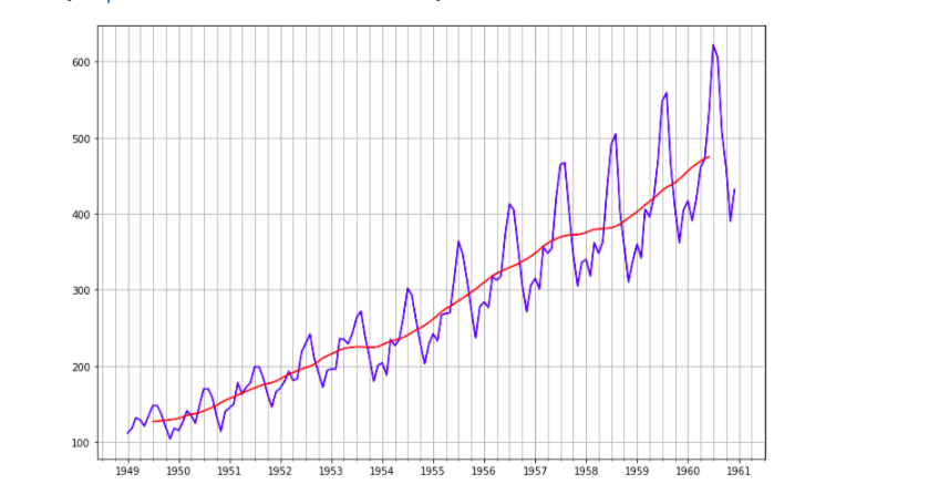
Again, we can see the trend is going up against the individual observations.

Conclusion

I hope this tutorial has helped you in understanding what Time Series is and how to get started with analyzing Time Series data.