Selecting Subsets of Data in Pandas: Part 1

This article is available as a Jupyter Notebook complete with exercises at the bottom to practice and detailed solutions in another notebook.

Intro to Data Science Bootcamp

For a more personalized class, take my Intro to Data Science Bootcamp. The next offering of this course is in Miami, on the

Part 1: Selection with [ ], .loc and .iloc

This is the beginning of a seven-part series on how to select subsets of data from a pandas DataFrame or Series. Pandas offers a wide variety of options for subset selection which necessitates multiple articles. This series is broken down into the following 7 topics.

1. Selection with a MultiIndex
2. Selecting subsets of data with methods
3. Selections with other Index types
4. Internals, Miscellaneous, and Conclusion

Assumptions before we begin

These series of articles assume you have no knowledge of pandas, but that you understand the fundamentals of the Python programming language. It also assumes that you have installed pandas on your machine.

The easiest way to get pandas along with Python and the rest of the main scientific computing libraries is to install the Anaconda distribution.

If you have no knowledge of Python then I suggest completing the following two books cover to cover before even touching pandas. They are both free.

The importance of making subset selections

You might be wondering why there needs to be so many articles on selecting subsets of data. This topic is extremely important to pandas and it’s unfortunate that it is fairly complicated because subset selection happens frequently during an actual analysis. Because you are frequently making subset selections, you need to master it in order to make your life with pandas easier.

I will also be doing a follow-up series on index alignment which is another extremely important topic that requires you to understand subset selection.

Always reference the documentation

The material in this article is also covered in the official pandas documentation on Indexing and Selecting Data. I highly recommend that you read that part of the documentation along with this tutorial. In fact, the documentation is one of the primary means for mastering pandas. I wrote a step-by-step article, How to Learn Pandas, which gives suggestions on how to use the documentation as you master pandas.

The anatomy of a DataFrame and a Series

The pandas library has two primary containers of data, the DataFrame and the Series. You will spend nearly all your time working with both of the objects when you use pandas. The DataFrame is used more than the Series, so let’s take a look at an image of it first.

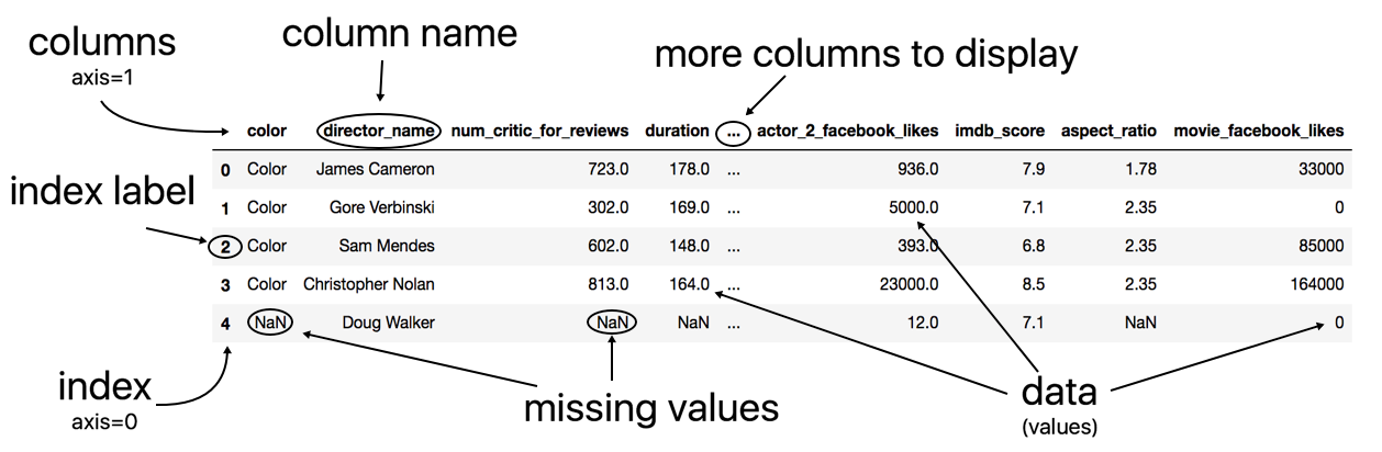
This image comes with some added illustrations to highlight its components. At first glance, the DataFrame looks like any other two-dimensional table of data that you have seen. It has rows and it has columns. Technically, there are three main components of the DataFrame.

The three components of a DataFrame

A DataFrame is composed of three different components, the index, columns, and the data. The data is also known as the values.

The index represents the sequence of values on the far left-hand side of the DataFrame. All the values in the index are in bold font. Each individual value of the index is called a label. Sometimes the index is referred to as the row labels. In the example above, the row labels are not very interesting and are just the integers beginning from 0 up to n-1, where n is the number of rows in the table. Pandas defaults DataFrames with this simple index.

The columns are the sequence of values at the very top of the DataFrame. They are also in bold font. Each individual value of the columns is called a column, but can also be referred to as column name or column label.

Everything else not in bold font is the data or values. You will sometimes hear DataFrames referred to as tabular data. This is just another name for a rectangular table data with rows and columns.

Axis and axes

It is also common terminology to refer to the rows or columns as an axis. Collectively, we call them axes. So, a row is an axis and a column is another axis.

The word axis appears as a parameter in many DataFrame methods. Pandas allows you to choose the direction of how the method will work with this parameter. This has nothing to do with subset selection so you can just ignore it for now.

Each row has a label and each column has a label

The main takeaway from the DataFrame anatomy is that each row has a label and each column has a label. These labels are used to refer to specific rows or columns in the DataFrame. It’s the same as how humans use names to refer to specific people.

What is subset selection?

Before we start doing subset selection, it might be good to define what it is. Subset selection is simply selecting particular rows and columns of data from a DataFrame (or Series). This could mean selecting all the rows and some of the columns, some of the rows and all of the columns, or some of each of the rows and columns.

Example selecting some columns and all rows

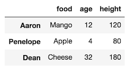
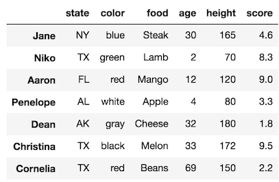
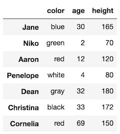
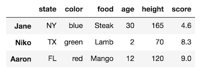
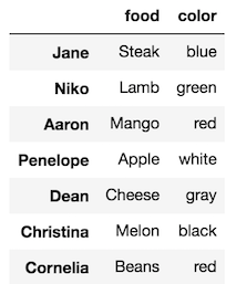
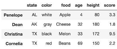
Let’s see some images of subset selection. We will first look at a sample DataFrame with fake data.

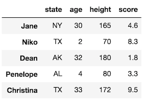
Let’s say we want to select just the columns color, age, and height but keep all the rows.

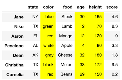
Our final DataFrame would look like this:

Example selecting some rows and all columns

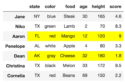
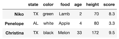
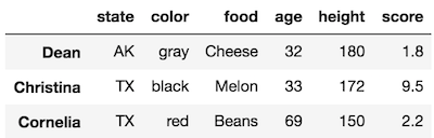
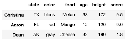
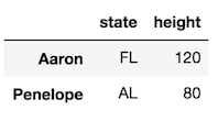
We can also make selections that select just some of the rows. Let’s select the rows with labels Aaron and Dean along with all of the columns:

Our final DataFrame would like:

Example selecting some rows and some columns

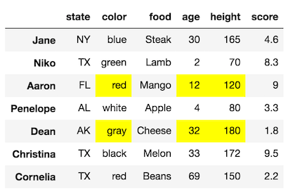
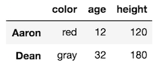
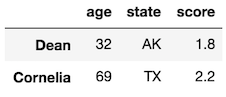
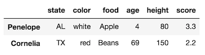
Let’s combine the selections from above and select the columns color, age, and height for only the rows with labels Aaron and Dean.

Our final DataFrame would look like this:

Pandas dual references: by label and by integer location

We already mentioned that each row and each column have a specific label that can be used to reference them. This is displayed in bold font in the DataFrame.

But, what hasn’t been mentioned, is that each row and column may be referenced by an integer as well. I call this integer location. The integer location begins at 0 and ends at n-1 for each row and column. Take a look above at our sample DataFrame one more time.

The rows with labels Aaron and Dean can also be referenced by their respective integer locations 2 and 4. Similarly, the columns color, age and height can be referenced by their integer locations 1, 3, and 4.

The documentation refers to integer location as position. I don’t particularly like this terminology as its not as explicit as integer location. The key thing term here is INTEGER.

What’s the difference between indexing and selecting subsets of data?

The documentation uses the term indexing frequently. This term is essentially just a one-word phrase to say ‘subset selection’. I prefer the term subset selection as, again, it is more descriptive of what is actually happening. Indexing is also the term used in the official Python documentation.

Focusing only on [], .loc, and .iloc

There are many ways to select subsets of data, but in this article we will only cover the usage of the square brackets ([]), .loc and .iloc. Collectively, they are called the indexers. These are by far the most common ways to select data. A different part of this Series will discuss a few methods that can be used to make subset selections.

If you have a DataFrame, df, your subset selection will look something like the following:

df[ ]df.loc[ ]df.iloc[ ]

A real subset selection will have something inside of the square brackets. All selections in this article will take place inside of those square brackets.

Notice that the square brackets also follow .loc and .iloc. All indexing in Python happens inside of these square brackets.

A term for just those square brackets

The term indexing operator is used to refer to the square brackets following an object. The .loc and .iloc indexers also use the indexing operator to make selections. I will use the term just the indexing operator to refer to df[]. This will distinguish it from df.loc[] and df.iloc[].

Read in data into a DataFrame with read_csv

Let’s begin using pandas to read in a DataFrame, and from there, use the indexing operator by itself to select subsets of data. All the data for these tutorials are in the data directory.

We will use the read_csv function to read in data into a DataFrame. We pass the path to the file as the first argument to the function. We will also use the index_col parameter to select the first column of data as the index (more on this later).

>>> import pandas as pd>>> import numpy as np

>>> df = pd.read_csv('data/sample_data.csv', index_col=0)>>> df

Extracting the individual DataFrame components

Earlier, we mentioned the three components of the DataFrame. The index, columns and data (values). We can extract each of these components into their own variables. Let’s do that and then inspect them:

>>> index = df.index>>> columns = df.columns>>> values = df.values

>>> indexIndex(['Jane', 'Niko', 'Aaron', 'Penelope', 'Dean', 'Christina',        'Cornelia'], dtype='object')

>>> columnsIndex(['state', 'color', 'food', 'age', 'height', 'score'],       dtype='object')

>>> valuesarray([['NY', 'blue', 'Steak', 30, 165, 4.6],       ['TX', 'green', 'Lamb', 2, 70, 8.3],       ['FL', 'red', 'Mango', 12, 120, 9.0],       ['AL', 'white', 'Apple', 4, 80, 3.3],       ['AK', 'gray', 'Cheese', 32, 180, 1.8],       ['TX', 'black', 'Melon', 33, 172, 9.5],       ['TX', 'red', 'Beans', 69, 150, 2.2]], dtype=object)

Data types of the components

Let’s output the type of each component to understand exactly what kind of object they are.

>>> type(index)pandas.core.indexes.base.Index

>>> type(columns)pandas.core.indexes.base.Index

>>> type(values)numpy.ndarray

Understanding these types

Interestingly, both the index and the columns are the same type. They are both a pandas Index object. This object is quite powerful in itself, but for now you can just think of it as a sequence of labels for either the rows or the columns.

The values are a NumPy ndarray, which stands for n-dimensional array, and is the primary container of data in the NumPy library. Pandas is built directly on top of NumPy and it's this array that is responsible for the bulk of the workload.

Beginning with just the indexing operator on DataFrames

We will begin our journey of selecting subsets by using just the indexing operator on a DataFrame. Its main purpose is to select a single column or multiple columns of data.

Selecting a single column as a Series

To select a single column of data, simply put the name of the column in-between the brackets. Let’s select the food column:

>>> df['food']Jane          SteakNiko           LambAaron         MangoPenelope      AppleDean         CheeseChristina     MelonCornelia      BeansName: food, dtype: object

Anatomy of a Series

Selecting a single column of data returns the other pandas data container, the Series. A Series is a one-dimensional sequence of labeled data. There are two main components of a Series, the index and the data(or values). There are NO columns in a Series.

The visual display of a Series is just plain text, as opposed to the nicely styled table for DataFrames. The sequence of person names on the left is the index. The sequence of food items on the right is the values.

You will also notice two extra pieces of data on the bottom of the Series. The name of the Series becomes the old-column name. You will also see the data type or dtype of the Series. You can ignore both these items for now.

Selecting multiple columns with just the indexing operator

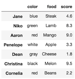
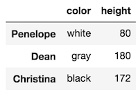
It’s possible to select multiple columns with just the indexing operator by passing it a list of column names. Let’s select color, food, and score:

>>> df[['color', 'food', 'score']]

Selecting multiple columns returns a DataFrame

Selecting multiple columns returns a DataFrame. You can actually select a single column as a DataFrame with a one-item list:

df[['food']]

Although, this resembles the Series from above, it is technically a DataFrame, a different object.

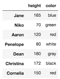
Column order doesn’t matter

When selecting multiple columns, you can select them in any order that you choose. It doesn’t have to be the same order as the original DataFrame. For instance, let’s select height and color.

df[['height', 'color']]

Exceptions

There are a couple common exceptions that arise when doing selections with just the indexing operator.

• If you misspell a word, you will get a KeyError
• If you forgot to use a list to contain multiple columns you will also get a KeyError

>>> df['hight']KeyError: 'hight'

>>> df['color', 'age'] # should be:  df[['color', 'age']]KeyError: ('color', 'age')

Summary of just the indexing operator

• Its primary purpose is to select columns by the column names
• Select a single column as a Series by passing the column name directly to it: df['col_name']
• Select multiple columns as a DataFrame by passing a list to it: df[['col_name1', 'col_name2']]
• You actually can select rows with it, but this will not be shown here as it is confusing and not used often.

Getting started with .loc

The .loc indexer selects data in a different way than just the indexing operator. It can select subsets of rows or columns. It can also simultaneously select subsets of rows and columns. Most importantly, it only selects data by the LABEL of the rows and columns.

Select a single row as a Series with .loc

The .loc indexer will return a single row as a Series when given a single row label. Let's select the row for Niko.

>>> df.loc['Niko']state        TXcolor     greenfood       Lambage           2height       70score       8.3Name: Niko, dtype: object

We now have a Series, where the old column names are now the index labels. The name of the Series has become the old index label, Niko in this case.

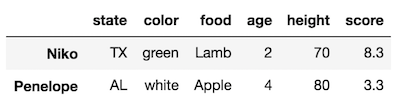
Select multiple rows as a DataFrame with .loc

To select multiple rows, put all the row labels you want to select in a list and pass that to .loc. Let's select Niko and Penelope.

>>> df.loc[['Niko', 'Penelope']]

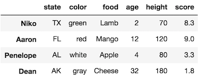
Use slice notation to select a range of rows with .loc

It is possible to ‘slice’ the rows of a DataFrame with .loc by using slice notation. Slice notation uses a colon to separate start, stop and step values. For instance we can select all the rows from Niko through Dean like this:

>>> df.loc['Niko':'Dean']

.loc includes the last value with slice notation

Notice that the row labeled with Dean was kept. In other data containers such as Python lists, the last value is excluded.

Other slices

You can use slice notation similarly to how you use it with lists. Let’s slice from the beginning through Aaron:

>>> df.loc[:'Aaron']

Slice from Niko to Christina stepping by 2:

>>> df.loc['Niko':'Christina':2]

Slice from Dean to the end:

>>> df.loc['Dean':]

Selecting rows and columns simultaneously with .loc

Unlike just the indexing operator, it is possible to select rows and columns simultaneously with .loc. You do it by separating your row and column selections by a comma. It will look something like this:

>>> df.loc[row_selection, column_selection]

Select two rows and three columns

For instance, if we wanted to select the rows Dean and Cornelia along with the columns age, state and score we would do this:

>>> df.loc[['Dean', 'Cornelia'], ['age', 'state', 'score']]

Use any combination of selections for either row or columns for .loc

Row or column selections can be any of the following as we have already seen:

• A single label
• A list of labels
• A slice with labels

We can use any of these three for either row or column selections with .loc. Let's see some examples.

Let’s select two rows and a single column:

>>> df.loc[['Dean', 'Aaron'], 'food']Dean     CheeseAaron     MangoName: food, dtype: object

Select a slice of rows and a list of columns:

>>> df.loc['Jane':'Penelope', ['state', 'color']]

Select a single row and a single column. This returns a scalar value.

>>> df.loc['Jane', 'age']30

Select a slice of rows and columns

>>> df.loc[:'Dean', 'height':]

Selecting all of the rows and some columns

It is possible to select all of the rows by using a single colon. You can then select columns as normal:

>>> df.loc[:, ['food', 'color']]

You can also use this notation to select all of the columns:

>>> df.loc[['Penelope','Cornelia'], :]

But, it isn’t necessary as we have seen, so you can leave out that last colon:

>>> df.loc[['Penelope','Cornelia']]

Assign row and column selections to variables

It might be easier to assign row and column selections to variables before you use .loc. This is useful if you are selecting many rows or columns:

>>> rows = ['Jane', 'Niko', 'Dean', 'Penelope', 'Christina']>>> cols = ['state', 'age', 'height', 'score']>>> df.loc[rows, cols]

Summary of .loc

• Only uses labels
• Can select rows and columns simultaneously
• Selection can be a single label, a list of labels or a slice of labels
• Put a comma between row and column selections

Getting started with .iloc

The .iloc indexer is very similar to .loc but only uses integer locations to make its selections. The word .iloc itself stands for integer location so that should help with remember what it does.

Selecting a single row with .iloc

By passing a single integer to .iloc, it will select one row as a Series:

>>> df.iloc[3]state        ALcolor     whitefood      Appleage           4height       80score       3.3Name: Penelope, dtype: object

Selecting multiple rows with .iloc

Use a list of integers to select multiple rows:

>>> df.iloc[[5, 2, 4]]       # remember, don't do df.iloc[5, 2, 4]

Use slice notation to select a range of rows with .iloc

Slice notation works just like a list in this instance and is exclusive of the last element

>>> df.iloc[3:5]

Select 3rd position until end:

>>> df.iloc[3:]

Select 3rd position to end by 2:

>>> df.iloc[3::2]

Selecting rows and columns simultaneously with .iloc

Just like with .iloc any combination of a single integer, lists of integers or slices can be used to select rows and columns simultaneously. Just remember to separate the selections with a comma.

Select two rows and two columns:

>>> df.iloc[[2,3], [0, 4]]

Select a slice of the rows and two columns:

>>> df.iloc[3:6, [1, 4]]

Select slices for both

>>> df.iloc[2:5, 2:5]