
Where did the least-square come from?
Where did the least-square come from?
What would you say in a machine learning interview, if asked about the mathematical basis of the least-square loss function?

Question: Why do you square the error in a regression machine learning task?
Ans: “Why, of course, it turns out all the errors (residuals) into positive quantities!”
Question: “OK, why not use a simpler absolute value function |x| to make all the errors positive?”
Ans: “Aha, you are trying to trick me. Absolute value function is not differentiable everywhere!”
Question: “That should not matter much for numerical algorithms. LASSO regression uses a term with absolute value and it can be handled. Also, why not 4th-power of x
Ans: Hmm…
A Bayesian argument
Remember that, for all tricky questions in machine learning, you can whip up a serious-sounding answer if you mix the word “Bayesian” in your argument.
OK, I was kidding there.
But yes, we should definitely have the argument ready about where popular loss functions like least-square and cross-entropy come from — at least when we try to find the most likely hypothesis for a supervised learning problem using Bayesian argument.
Read on…
The Basics: Bayes Theorem and the ‘Most Probable Hypothesis’
Bayes’ theorem is probably the most influential identity of probability theory for modern machine learning and artificial intelligence systems. For a super intuitive introduction to the topic, please see this great tutorial by Brandon Rohrer. I will just concentrate on the equation.


This essentially tells that you update your belief (prior probability) after seeing the data/evidence (likelihood) and assign the updated degree of belief to the term posterior probability. You can start with a belief, but each data point will either strengthen or weaken that belief and you update your hypothesis all the time.

Let us now recast the Bayes’ theorem in different symbols — symbols pertaining to data science. Let us denote, data by D and hypothesis by h. This means we apply Bayes’ formula to try to determine what hypothesis the data came from, given the data. We rewrite the theorem as,

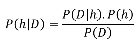
Now, in general, we have a large (often infinite) hypothesis space i.e. many hypotheses to choose from. The essence of Bayesian inference is that we want to examine the data to maximize the probability of one hypothesis which is most likely to give rise to the observed data. We basically want to determine argmax of the P(h|D)i.e. we want to know which h is most probable, given the observed D.
A shortcut trick: Maximum Likelihood
The equation above looks simple but it is notoriously tricky to compute in practice — because of extremely large hypothesis space and complexity in evaluating integrals over complicated probability distribution functions.
However, in the quest of our search for the ‘most probable hypothesis given data,’ we can simplify it further.
- We can drop the term in the denominator it does not have any term containing h i.e. hypothesis. We can imagine it as a normalizer to make total probability sum up to 1.
- Uniform prior assumption— this essentially relaxes any assumption on the nature of P(h) by making it uniform i.e. all hypotheses are probable. Then it is a constant number 1/|Vsd| where |Vsd| is the size of the version space i.e. a set of all hypothesis consistent with the training data. Then it does not actually figure in the determination of the maximally probable hypothesis.
After these two simplifying assumptions, the maximum likelihood (ML) hypothesis can be given by,
This simply means the most likely hypothesis is the one for which the conditional probability of the observed data (given the hypothesis) reaches maximum.
Next piece in the puzzle: Noise in the data
We generally start using least-square error while learning about simple linear regression back in Stats 101 but this simple-looking loss function resides firmly inside pretty much every supervised machine learning algorithm viz. linear models, splines, decision trees, or deep learning networks.
So, what’s special about it? Is it related to the Bayesian inference in any way?
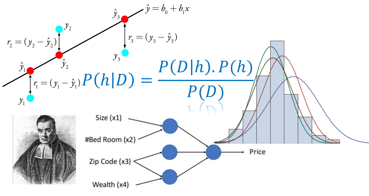
It turns out that, the key connection between the least-square error and Bayesian inference is through the assumed nature of the error or residuals.
Measured/observed data is never error-free and there is always random noise associated with data, which can be thought of the signal of interest. Task of a machine learning algorithm is to estimate/approximate the function which could have generated the data by separating the signal from the noise.
But what can we say about the nature of this noise? It turns out that noise can be modeled as a random variable. Therefore, we can associate a probability distribution of our choice to this random variable.
One of the key assumptions of least-square optimization is that probability distribution over residuals is our trusted old friend — Gaussian Normal.
This means that every data point (d) in a supervised learning training data set can be written as the sum of the unknown function f(x) (which the learning algorithm is trying to approximate) and an error term which is drawn from a Normal distribution of zero mean (μ) and unknown variance σ². This is what I mean,

And from this assertion, we can easily derive that the maximum likely hypothesis is the one which minimizes the least-square error.
Math warning: There is no way around some bit of math to formally derive the least-square optimization criteria from the ML hypothesis. And there is no good way to type in math in Medium. So, I have to paste an image to show the derivation. Feel free to skip this section, I will summarize the key conclusion in the next section.