Materials covered in Part 4:

In this story, I’m going to cover the followings. In Part 1–3 we already covered the basics and from here on, the topics will be based on the fundamentals that we already learned.

• Projections
• Orthonormal vectors
• Orthogonal matrix
• Gram Schmidt process

The corresponding lectures from the videos by Dr. Gilbert Strang for these topics are Lectures 15–17 and I would recommend you actually watch his talks for better understanding of the materials!

Introduction to Projections

First, let’s talk about “projections”. Projection is a linear transformation from a vectorspace to itself. Let’s take a look at a simple example. In 2D plane, you have two vectors “a” and “b”. You want to know the vector “b” that’s projected on to the vector “a”. Let’s call this projected vector “p

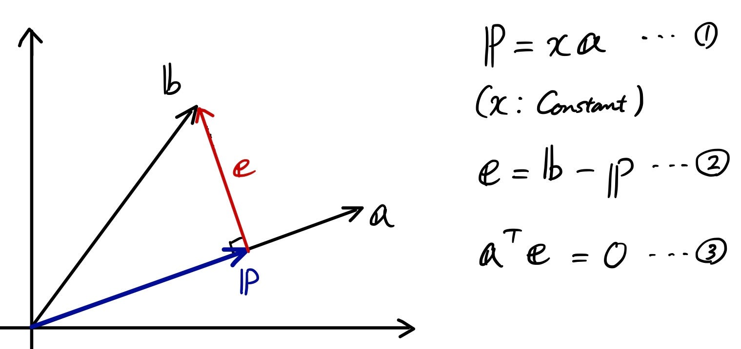
OK, so the first goal here is to figure out “x” so that using the 1st equation, you can represent “p” as something times “a”. Try taking sometime solving the equations.

Here’s the answer.

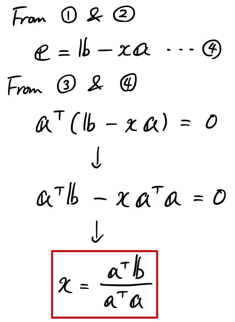
Now you know “x”, so put this in the 1st equation to see what “p” is. Since “x” is a constant, we could tweak it a little to modify the equation so that “p” is represented by “something” times the vector “b”.

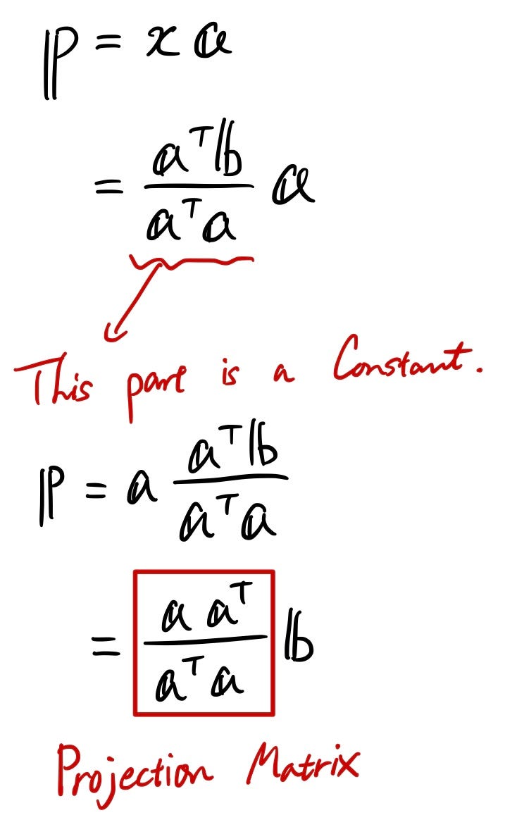
So now we have this “Projection Matrix”. It might be difficult to fully understand from this equation form, so let me give you a concrete example below:

Let’s say you have two vectors.

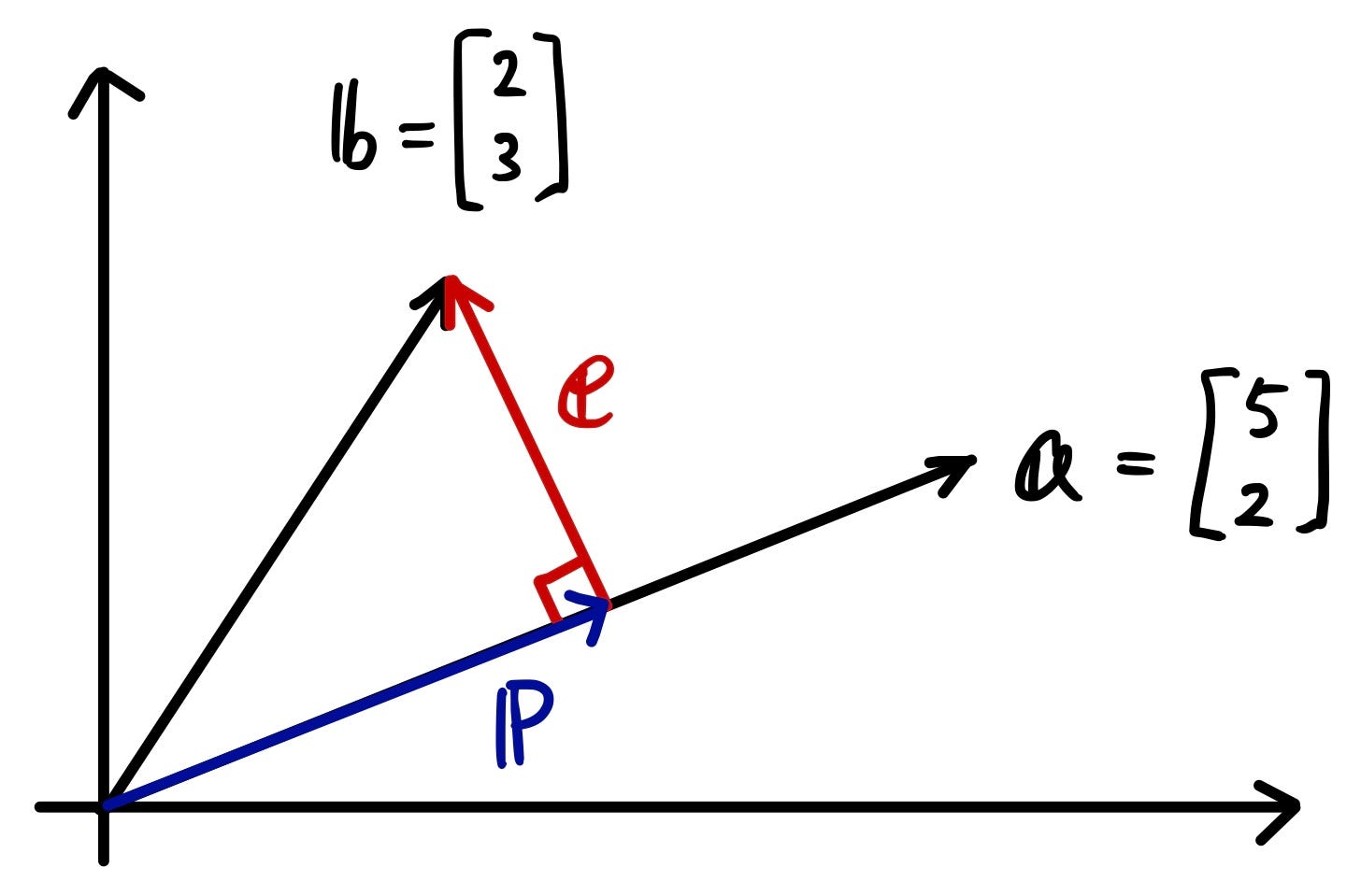
Just like what we did before when deriving the equation for projection, we will do the same with actual vectors.

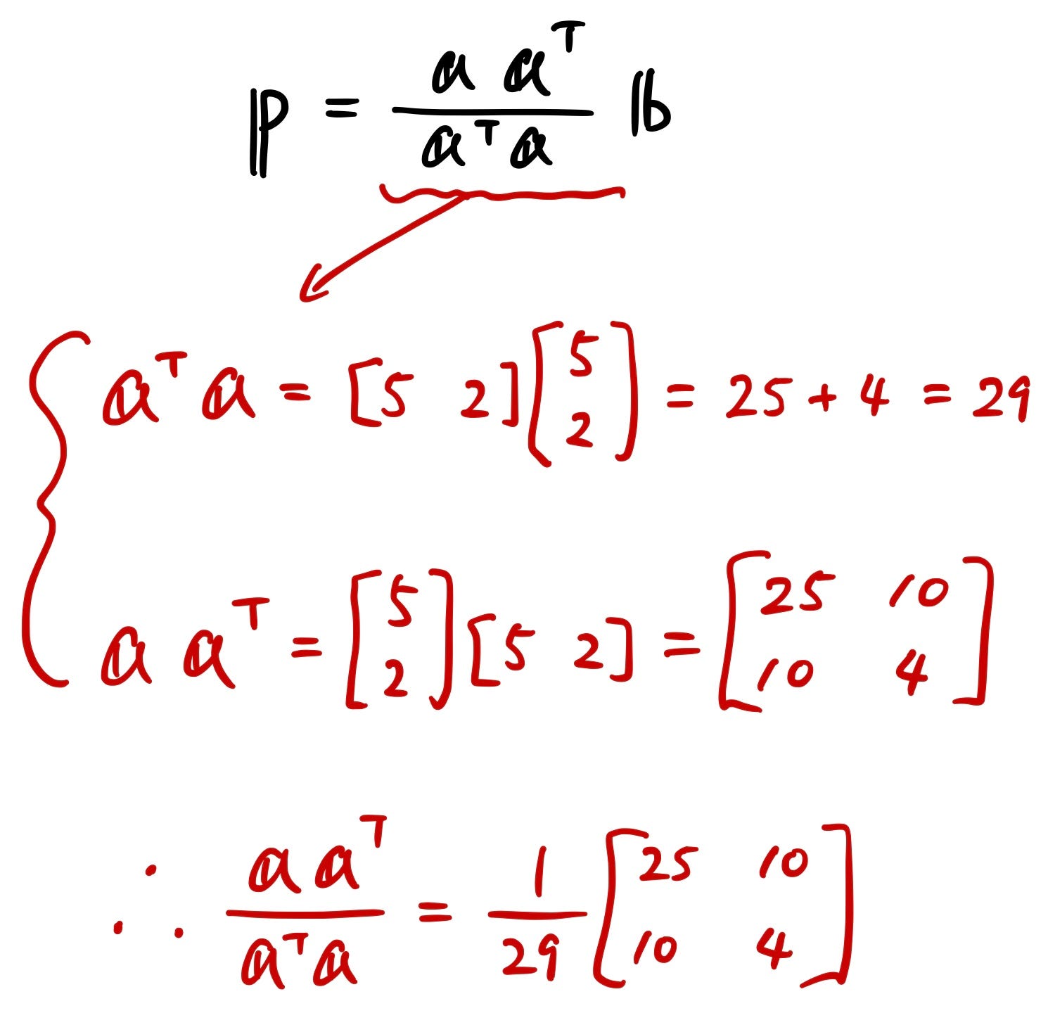
Now using this calculated projection matrix, we can figure out the projected vector “p”.

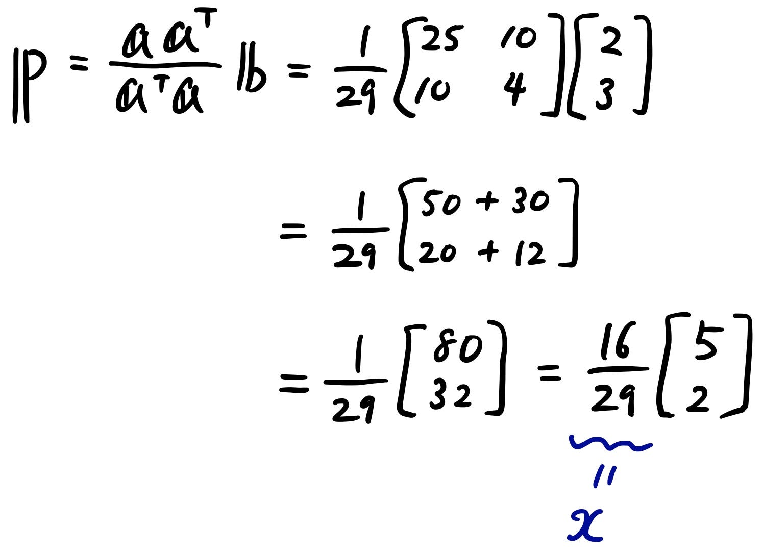
Now you can see that the projected vector “p” is nothing but the scaled version of a vector “a”. Remember that a = transpose[5, 2]? It makes sense because the projected vector is on the vector “a”.

Now let’s take a look at a 3D example.

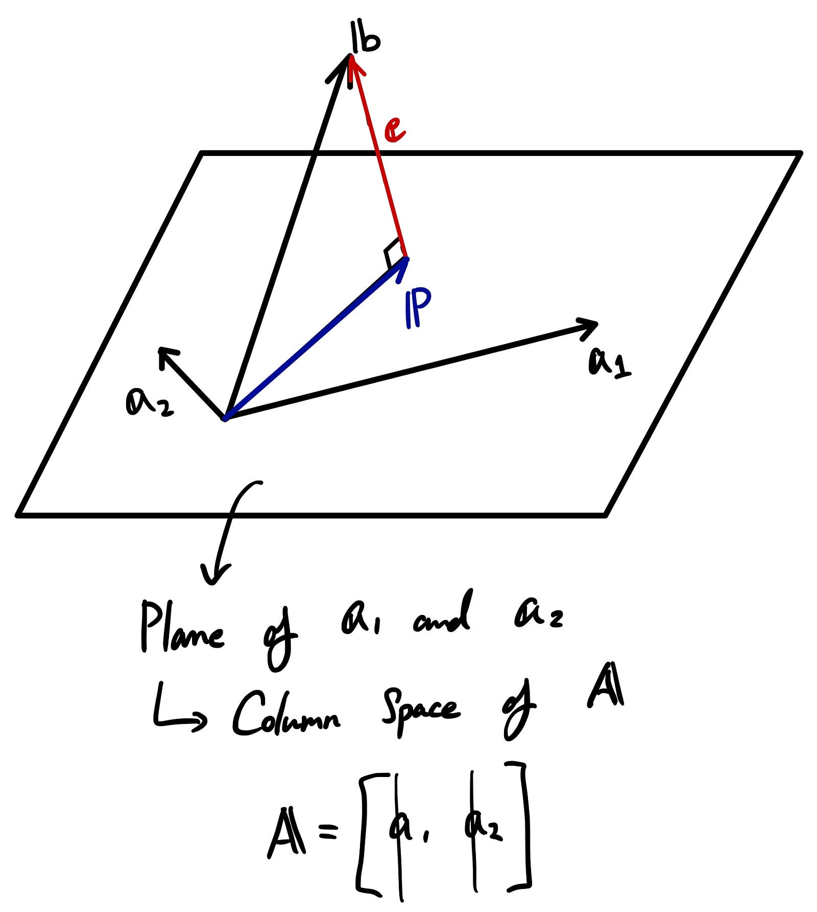
The plane you see there is a column space represented by column vectors “a1” and “a2”. “A” is a matrix that has those column vectors in there. Now what we want to do is to project vector “b”, which is not on this plane, to the plane.

Just like what we did in the 2D example, we define two vectors “p” and “e”.

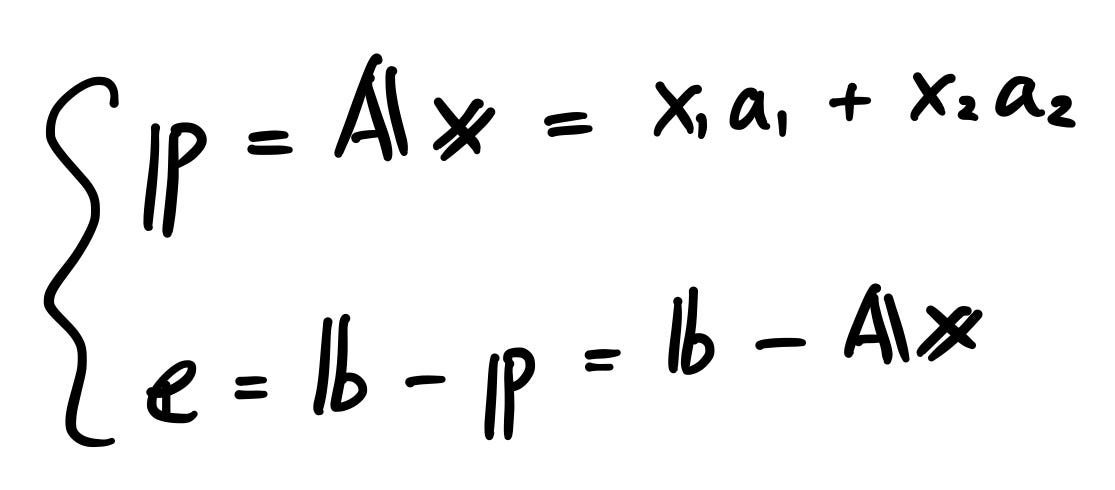
Since “e” is perpendicular to the plane, we can create two equations as follows. By combing those two equations and modifying it accordingly, we get the scaling factor “x”.

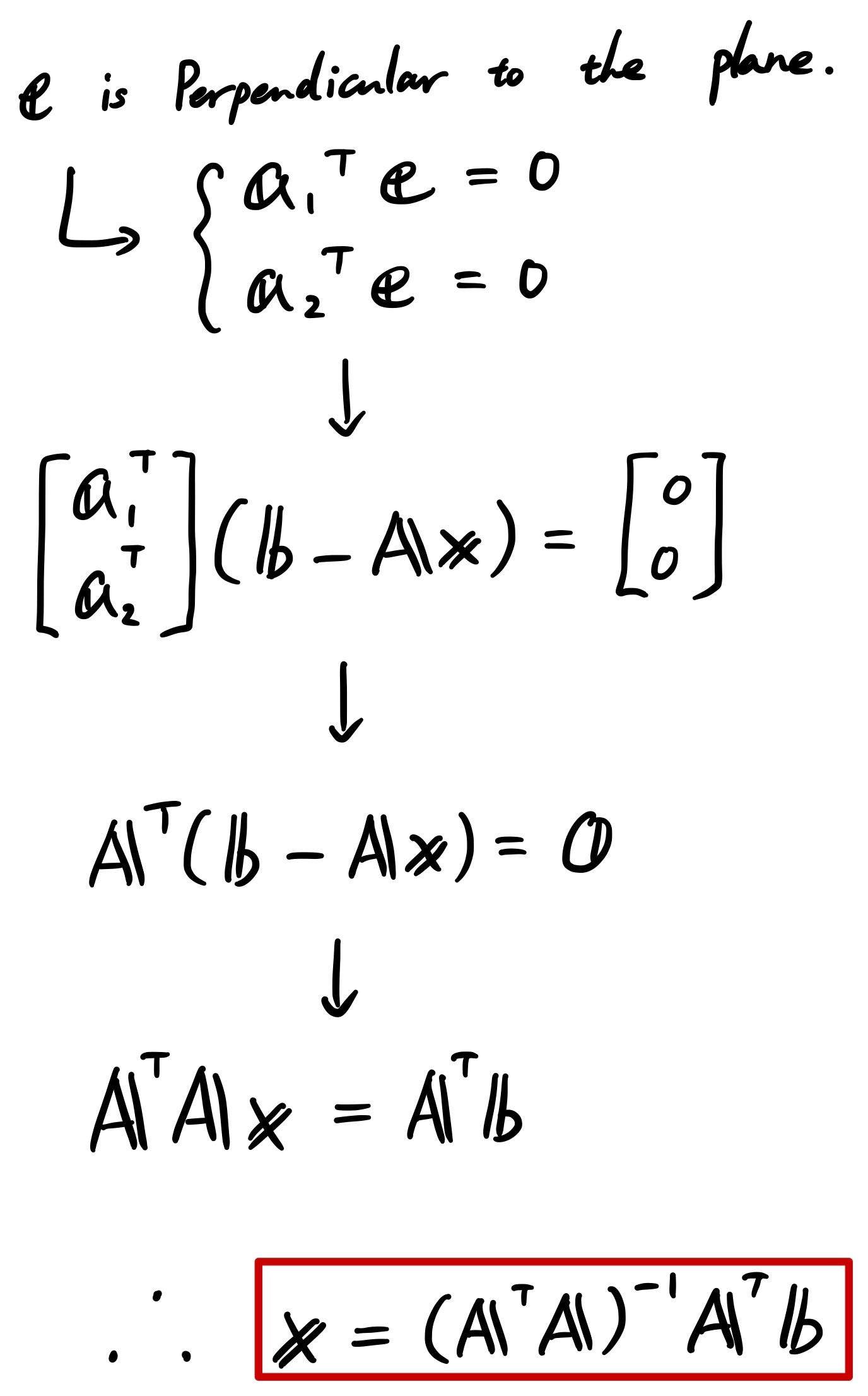
Using the above scaling factor, we can get “p”.

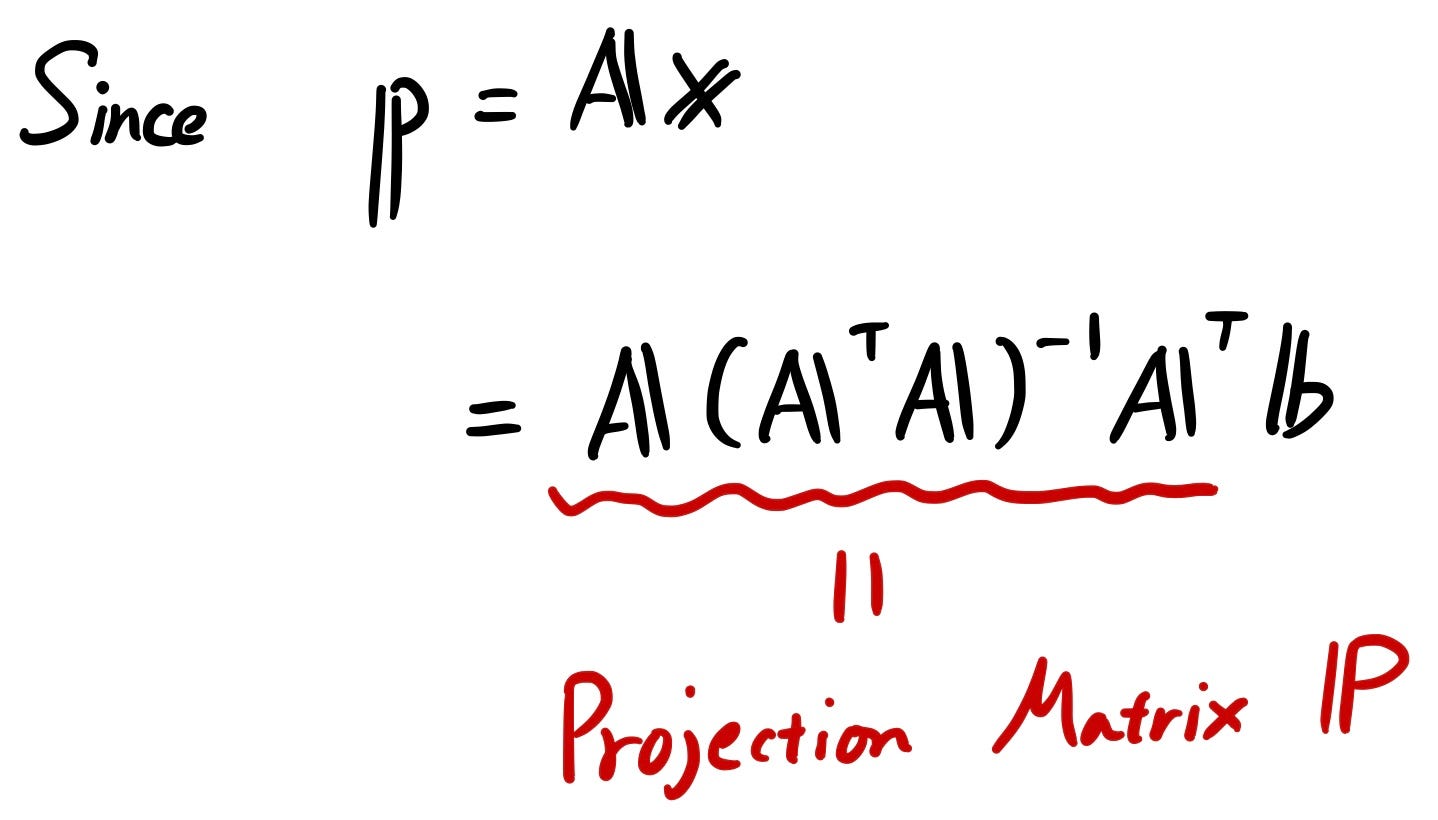
Now we get the “Projection Matrix”! This time, it’s a more general form so that it could be used for dimensions more than 3.

Let’s take a look at the properties.

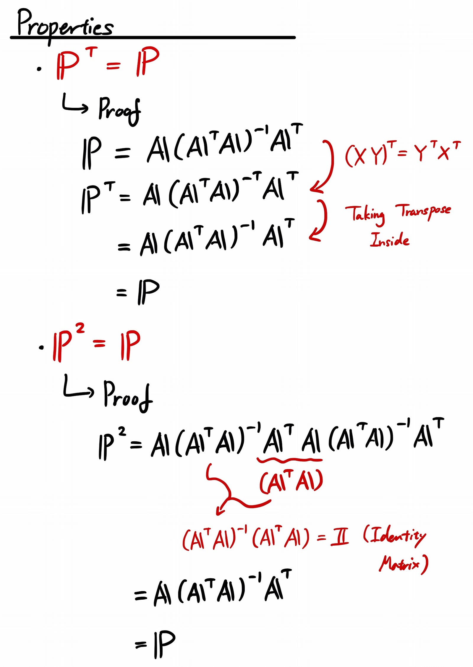
This projection part is very important so make sure you understand it well! It’s used to derive the formula for many of the algorithms used in Machine Learning. To give you an example, a well know machine learning technique called “Support Vector Machine (SVM)” when calculating the margin. If you know what I’m talking about, great! If not, that’s ok. I will cover this topic as well sometime in the future.

Introduction to Orthonormal vectors

Now another new topic called “Orthonormal vectors”. It’s very simple. If two of the vectors are:

1. Unit vectors
2. Orthogonal to each other

Then they are orthonormal vectors. In equations, it’s expressed as something like the following:

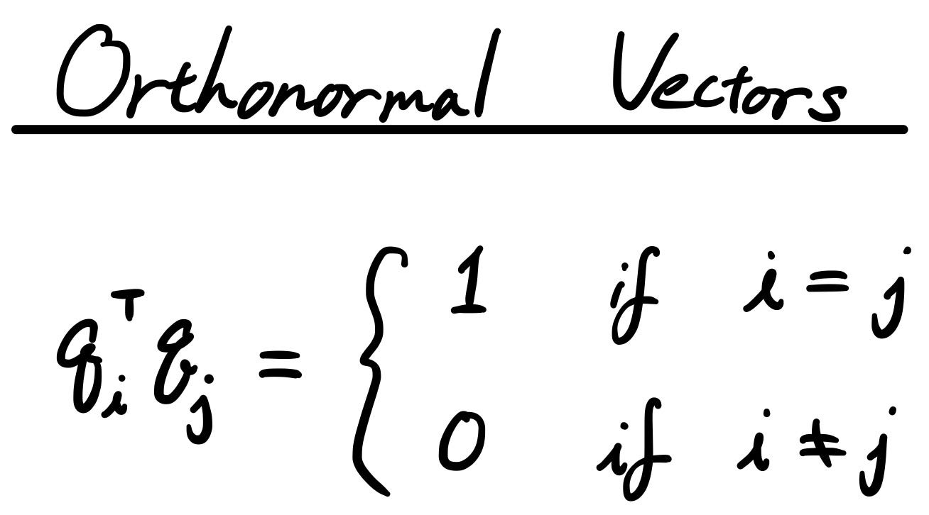
We covered orthogonality in Part 3. It’s basically saying that two of the vectors are perpendicular to each other, or the dot product is zero.

Here, I’m going to introduce you to the unit vector. It’s just normalizing the vector so that the length of the unit vector is always 1.

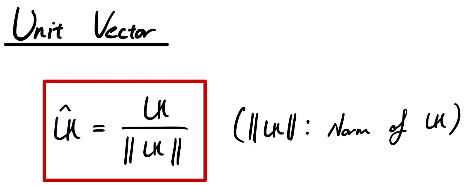
As an example, if you have a vector like the one below, the unit vector can be calculated accordingly.

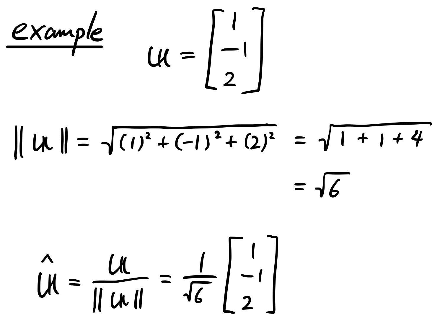
So just to summarize, orthonormal vectors are vectors that are orthogonal to each other and are also unit vectors.

Introduction to Orthogonal matrix

“Orthogonal Matrix” is nothing but the square matrix whose rows and columns are orthonormal vectors.

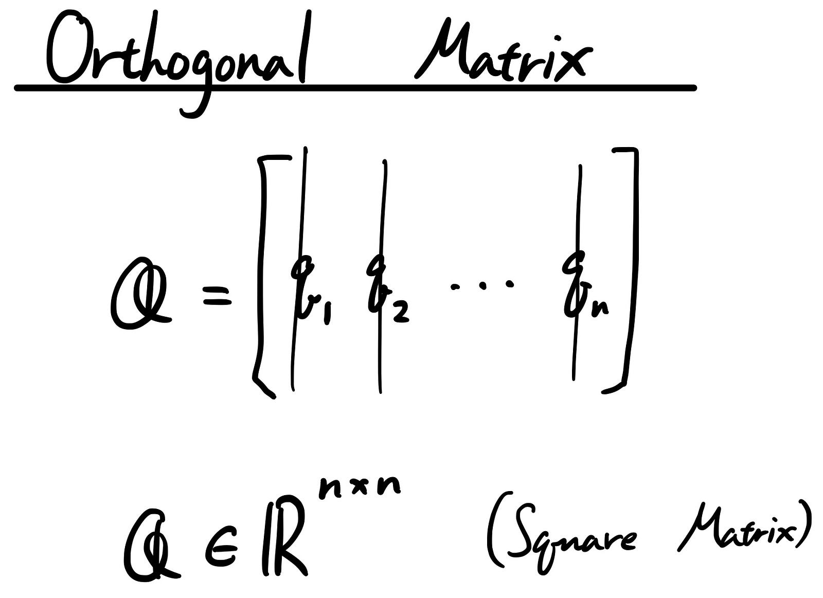
Orthogonal matrix has an interesting property that multiplied by its own transpose, the result becomes an identity matrix. Therefore, we can say that the transpose of the orthogonal matrix is equal to the inverse of the orthogonal matrix. This property is very important when it comes to eigen decomposition and singular value decomposition (covered in the later stories) so keep that in mind!

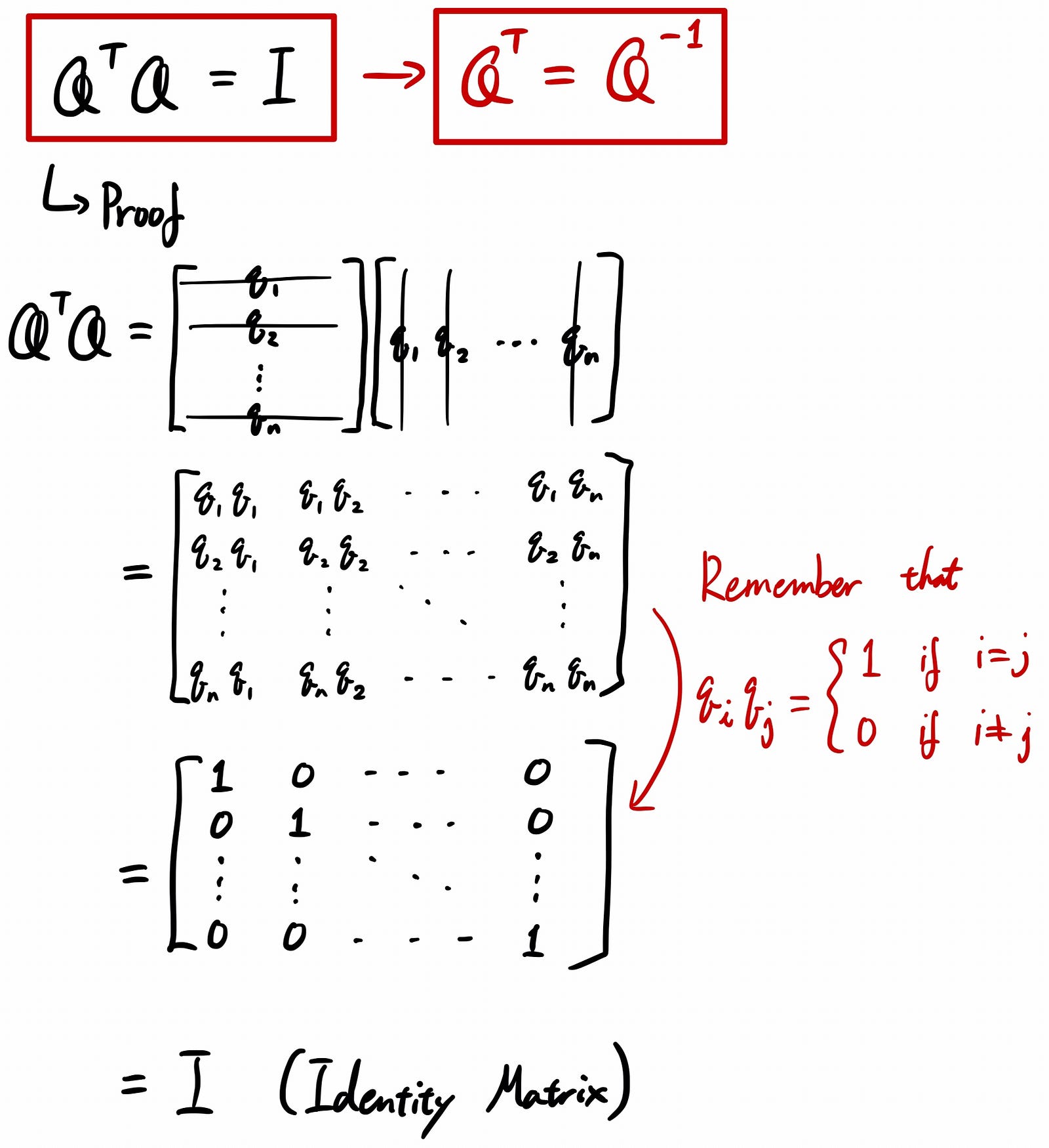
Above is just showing what multiplying with its own transpose makes it an identity matrix.

Introduction to Gram-Schmidt process

So, let’s say you have a bunch of vectors, but they are not orthonormal vectors. You want to turn them into orthonormal vectors, but how can we do that? This is where “Gram-Schmidt Process” comes into play.

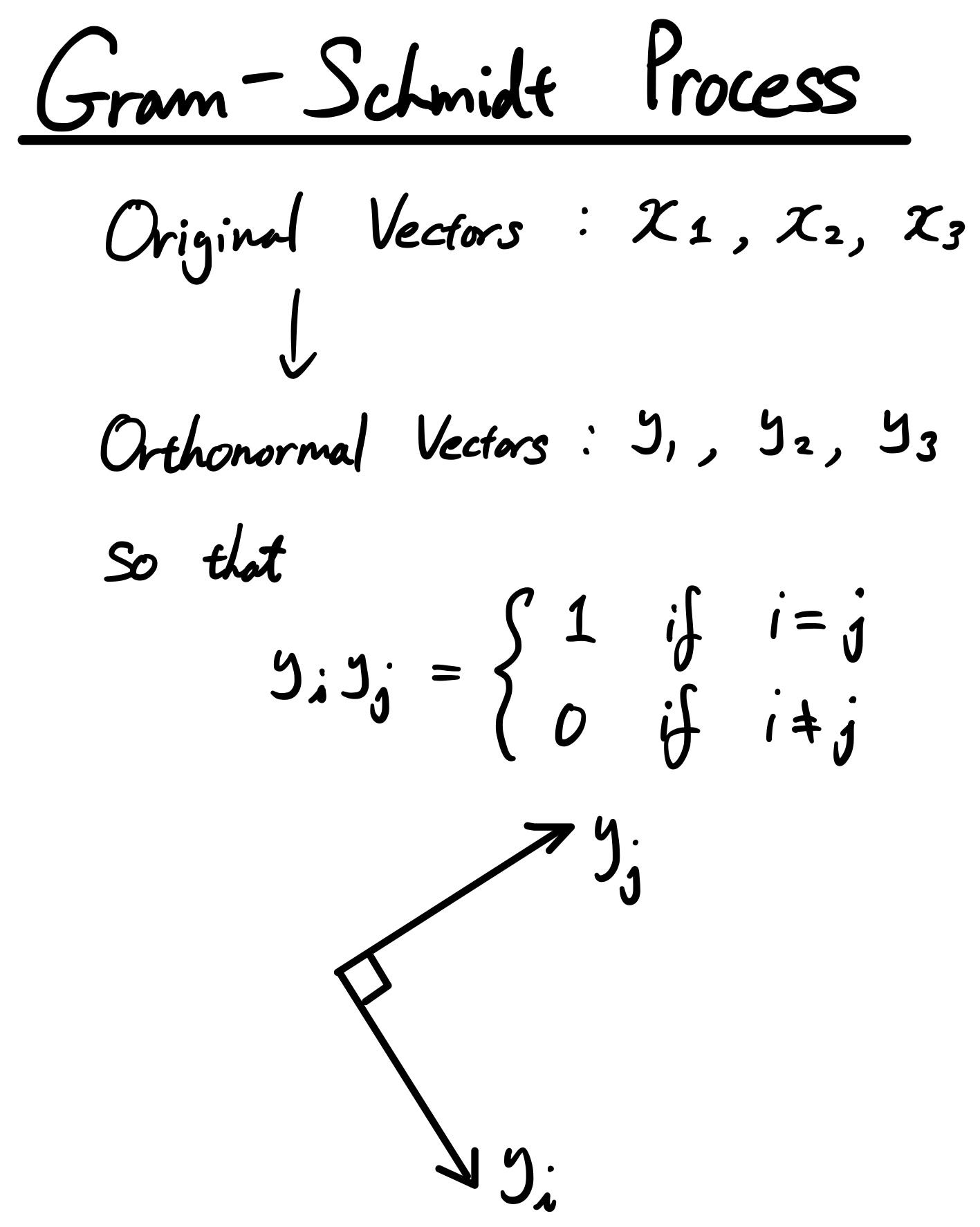
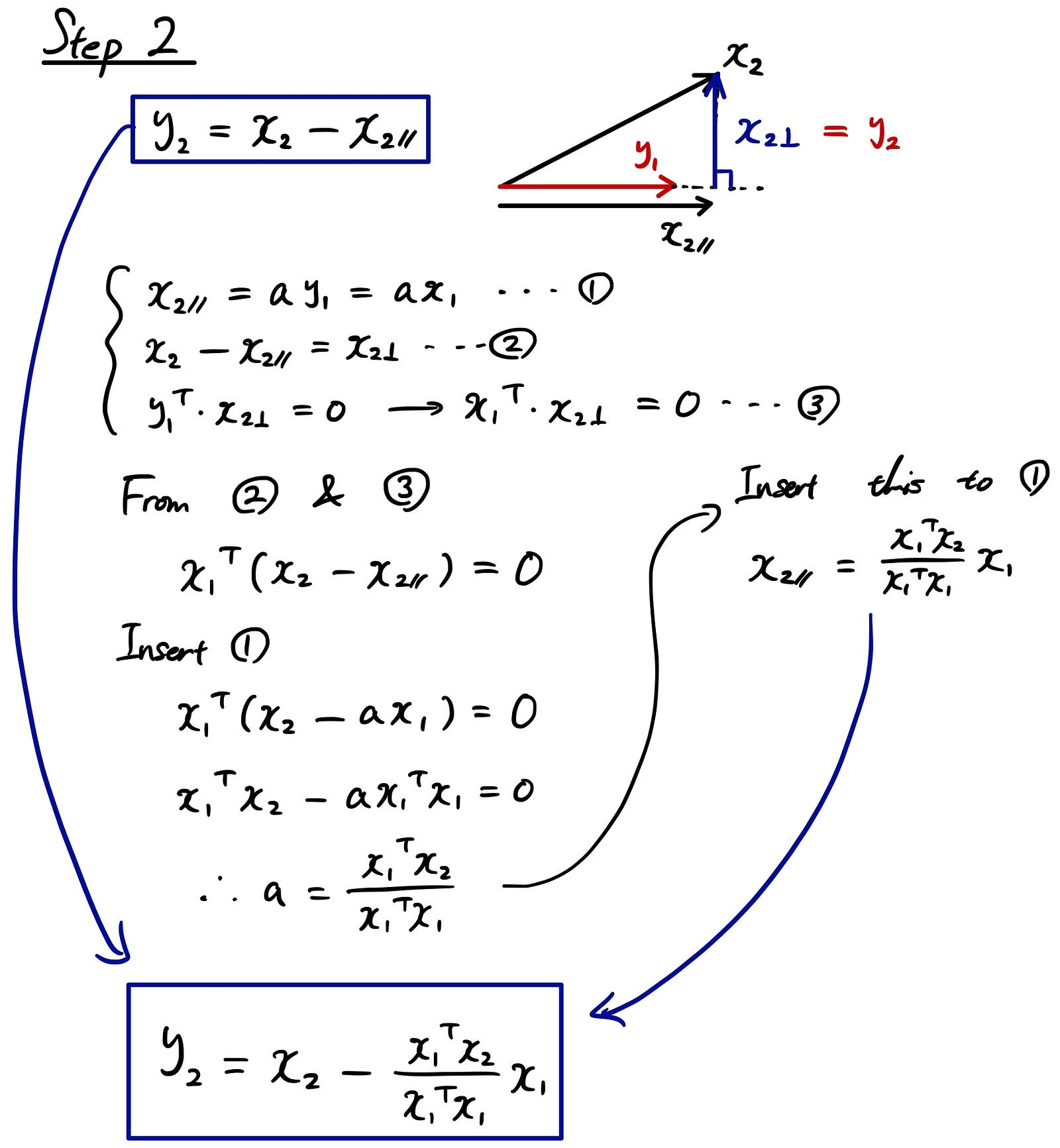
Let’s take a step by step example of how the process works. The 1st step is very simple. You just assign your vector to be “y1”. Later, you are going to convert all these y’s to unit vectors, but first let’s deal with the orthogonality.

From Step 2, this is where the actual process comes into play. So we want the outcome vectors to be orthogonal to each other. Look at the triangle plot below. We already defined “y1” and now we want the vector “y2” that’s orthogonal to “y1”, but derived from the original vector “x2”. If we decompose “x2” to parallel and perpendicular vectors, the only vector that we want in the end is the one that’s perpendicular. That’s why we are subtracting the parallel version of the “x2” from the original vector “x2”.

Let’s take a look at the 3rd step.

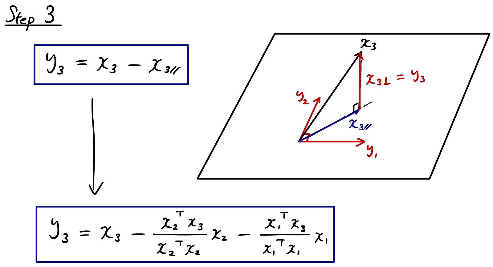
By now, you might have noticed the patterns here.

If we generalize the pattern, the Gram-Schmidt Process is described as follows.

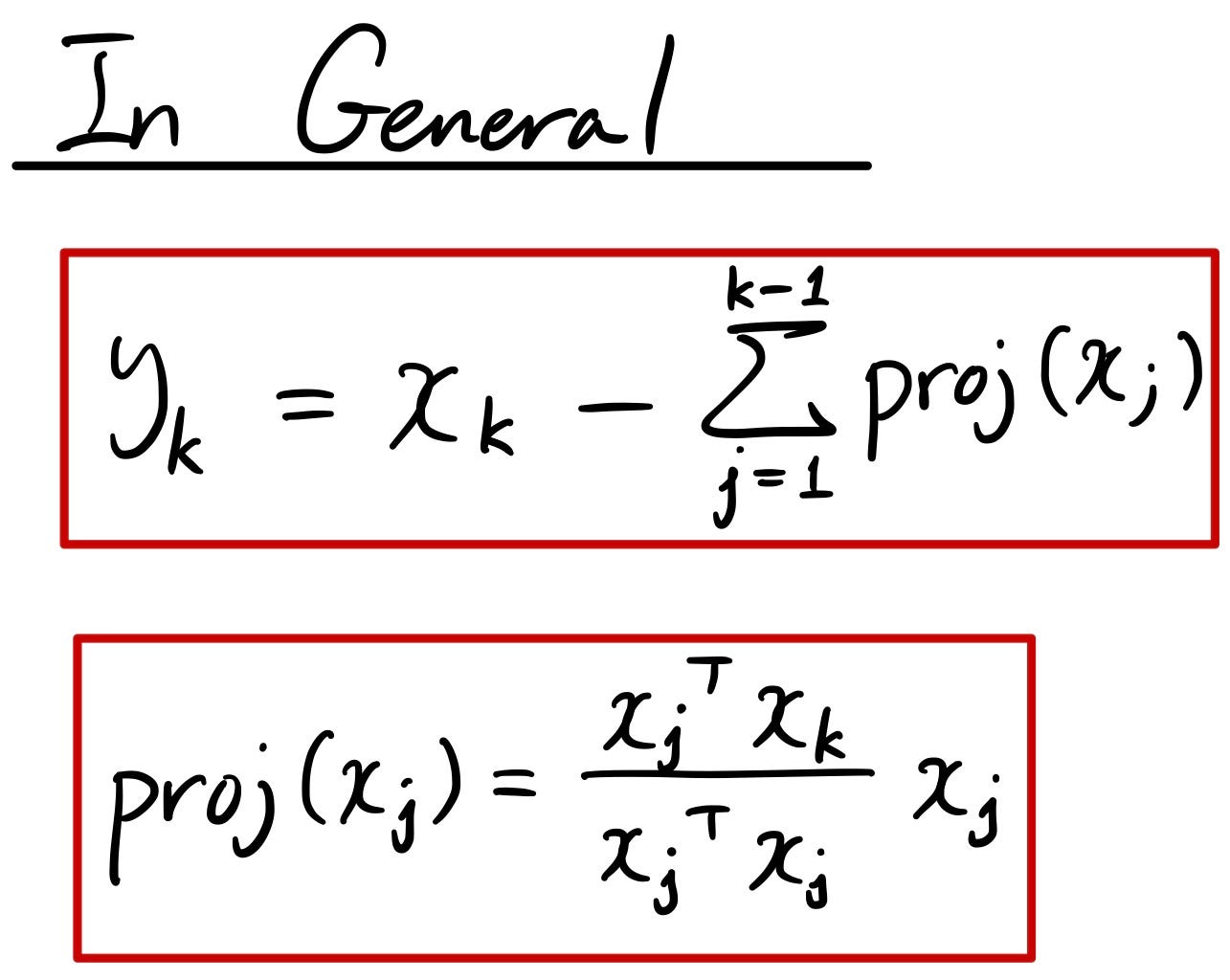
In the end, don’t forget to normalize to unit vectors!