Materials covered in Part 3:

In this article, we are going to cover some more fundamental concepts in linear algebra. This will be the last to cover the fundamentals and we will move on to a more advanced concepts in linear algebra from next article where all the of the fundamentals that we covered so far in Part 1–3 will be combined. So please be advised to understand what we studied so far!

• Linear independence
• Span
• Basis
• 4 fundamental subspaces
• Orthogonality

Introduction to linear independence

First, let’s talk about “linear independence”. We say vectors are independent when no linear combinations of them gives zero vector except when all the coefficients are zeros. If we were to write this in equations, it looks like below:

where x’s are vectors, c’s are coefficients. Even if you could think of one combination that could make the equation zero, then the vectors are not independent.

Let’s take an example to understand this concept.

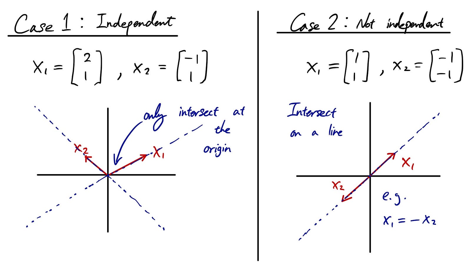
Case 1 is independent case where two of the vectors that we are considering are independent from each other. This means that the only intersection between those two vectors are at the origin. This only occurs when we multiply both vectors with 0 (zero).

On the other hand, case 2 is not independent. We can find numerous pairs of coefficients for intersections. It could be c1 = 1 and c2 = -1 as in the example above so that x1 = -x2. It could be -x1 = x2 with c1 = -1 and c2 = 1. Since we can find coefficients with non-zeros that could make vectors cancel each other out, we call these cases not independent.

Introduction to span

We say vectors span a space when the space consists of all linear combinations of the vectors.

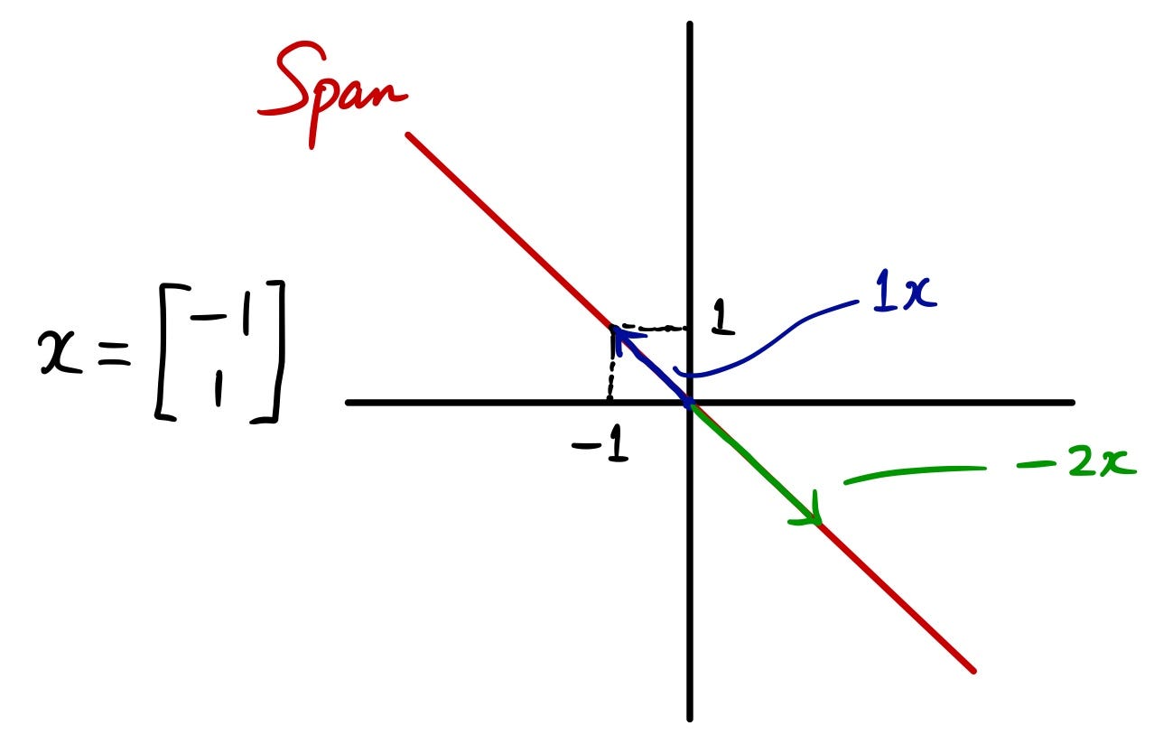
Let’s take a look at an easy example. Let’s say you have a vector x as follows. The span of this vector is the red line represented in the figure:

Why? Because if you think about all the linear combination, we can take any coefficient on x. It could be 1 or -2, 5 or 2.3, anything. But if you draw that points represented by different coefficients, it all lies on the red line. Basically, we are spanning out the vector to see what kind of space it gives us. This is span in linear algebra.

Introduction to basis

Now you know linear independence and span. Next, let’s introduce you to another new concept called “basis”.

Basis by its definition is very easy to understand if you understand the concepts I just explained.

Basis for a space is a sequence of vectors that are:

1. Linearly independent
2. Span the space

For example, basis can be something like below:

For “span” and “basis”, there’s an awesome video visualizing these concepts and I strongly recommend you watch this at least 2 times!

The video is part of the video series: “Essence of linear algebra” by 3Blue1Brown so feel free to take some time watching all the videos. They are amazing!

Introduction to 4 fundamental subspaces

Let’s try to combine some of the concepts that we have already learned to tie the knowledge with each other. Here, I’m going to explain about 4 fundamental subspaces:

1. Column space
2. Nullspace
3. Row space
4. Left nullspace

We’ve already studied each of these subspaces in the previous articles. But here, I’m trying to tie each of those concepts together based on dimensions.

I hope you remember what “rank” is. If not, please go back to Part 2 to check it out again. In short, rank is equal to the number of pivots in a matrix. We call it “full rank” when the rank is equal to the maximum dimension (row or column, whichever is smaller) of a matrix. We call it “rank deficient” if the matrix is not full rank.

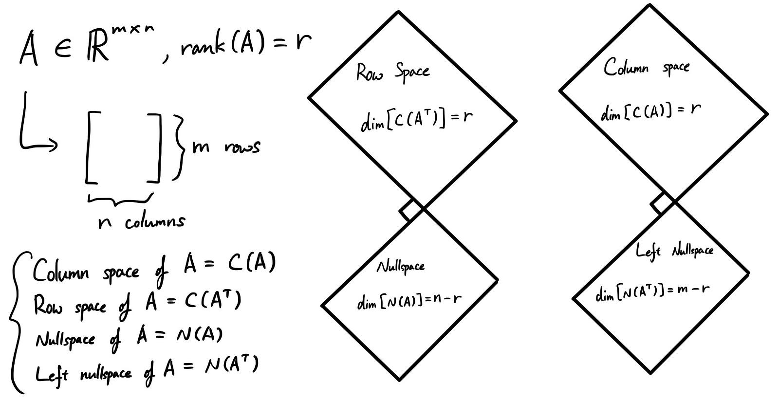
Here, we are looking at some rank deficient case. Suppose the rank of a matrix is “r” and you have “m” rows and “n” columns.

When we think about row space, the rank of row space is “r” since this is the number of pivots we have. But remember when we talked about free variables last time? Since we are thinking about rank deficient case, n > r. This means that there are some free variables in the matrix! Of course they are in nullspace, so the dimension of the nullspace = the number of free variables = n - r.

Same goes for the column space. Except in this case, to differentiate between row’s nullspace, we call the nullspace for column space, “left nullspace”.

Introduction to orthogonality

OK, it was quite a long way, but here comes the last fundamental concepts you need to learn. This concept is also very important and at the same time, very useful so let’s try to understand this completely!

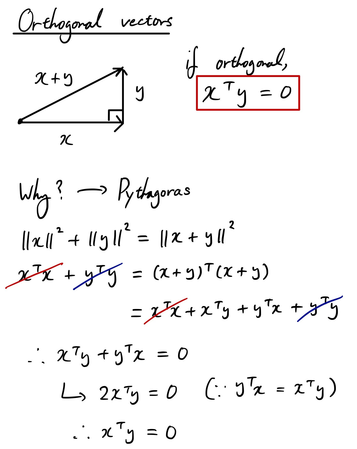
First, let’s start off with the definition and why it becomes like that.

That was pretty easy! So for the Pythagoras equation to be satisfied, we need the equation covered in the red box to be satisfied. This is the equation to show orthogonality and it’s pretty useful since we can wipe off the term that’s orthogonal when calculating a complex equation.