因為我用的版本是python3.6.0，而示例程式碼似乎是python2版本的，於是遇到一些問題。

示例程式碼是ipynb格式的，開啟方式：cmd下執行ipython notebook, 在瀏覽器中開啟網頁（如下），可以點選Upload按鈕選擇要開啟的檔案。

但是程式碼是一行一行的，怎麼在spyder裡面直接執行呢？

如圖2點選儲存為python格式的就可以在spyder裡面打開了。

一執行發現報錯了，原來資料集沒有下載：

回頭看作業頁面的說明，原來說了要怎麼下載的：

但是這個是Shell命令。（windows10上可以啟用linux子系統）開啟bash，輸入命令，開始下載CIFAR-10 dataset

：

執行程式碼的時候報了許多錯，其中之一是pickle.load反序列化，

  File "E:\assignment1\cs231n\data_utils.py", line 9, in load_CIFAR_batch
    datadict = pickle.load(f)

UnicodeDecodeError: 'ascii' codec can't decode byte 0x8b in position 6: ordinal not in range(128)

查到別人的解答，點選開啟連結

with open(filename, 'rb') as f:
    datadict = pickle.load(f,encoding='iso-8859-1')
 

我們需要告訴pickle：how to convert python bytestring data to Python 3 strings，The default is to try and decode all string data as ASCII

填補程式碼說明：

1. 交叉驗證選擇最佳的K值

# In[ ]:


num_folds = 5
k_choices = [1, 3, 5, 8, 10, 12, 15, 20, 50, 100]

X_train_folds = []
y_train_folds = []
################################################################################
# TODO:                                                                        #
# Split up the training data into folds. After splitting, X_train_folds and    #
# y_train_folds should each be lists of length num_folds, where                #
# y_train_folds[i] is the label vector for the points in X_train_folds[i].     #
# Hint: Look up the numpy array_split function.                                #
################################################################################
X_train_folds=np.array_split(X_train,num_folds)
y_train_folds=np.array_split(y_train,num_folds)
################################################################################
#                                 END OF YOUR CODE                             #
################################################################################

# A dictionary holding the accuracies for different values of k that we find
# when running cross-validation. After running cross-validation,
# k_to_accuracies[k] should be a list of length num_folds giving the different
# accuracy values that we found when using that value of k.
k_to_accuracies = {}


################################################################################
# TODO:                                                                        #
# Perform k-fold cross validation to find the best value of k. For each        #
# possible value of k, run the k-nearest-neighbor algorithm num_folds times,   #
# where in each case you use all but one of the folds as training data and the #
# last fold as a validation set. Store the accuracies for all fold and all     #
# values of k in the k_to_accuracies dictionary.                               #
################################################################################
for k in k_choices:
    k_to_accuracies[k] = np.zeros(num_folds)
    for i in range(num_folds):
        Xtr = np.array(X_train_folds[:i] + X_train_folds[i+1:])#把訓練集中的一塊劃為驗證集
        ytr = np.array(y_train_folds[:i] + y_train_folds[i+1:])
        Xte = np.array(X_train_folds[i])
        yte = np.array(y_train_folds[i])     

        Xtr = np.reshape(Xtr, (X_train.shape[0]/ 5*4, -1))
        ytr = np.reshape(ytr, (y_train.shape[0]/ 5*4, -1))
        Xte = np.reshape(Xte, (X_train.shape[0] / 5, -1))
        yte = np.reshape(yte, (y_train.shape[0] / 5, -1))

        classifier.train(Xtr, ytr)
        yte_pred = classifier.predict(Xte, k)
        yte_pred = np.reshape(yte_pred, (yte_pred.shape[0], -1))
        num_correct = np.sum(yte_pred == yte)
        accuracy = float(num_correct) / len(yte)
        k_to_accuracies[k][i] = accuracy

        
################################################################################
#                                 END OF YOUR CODE                             #
################################################################################

# Print out the computed accuracies
for k in sorted(k_to_accuracies):
    for accuracy in k_to_accuracies[k]:
        print ('k = %d, accuracy = %f' % (k, accuracy))
 

這裡使用的是交叉驗證(cross-validation)去獲取knn中的超引數K的最佳值，其基本思想是，將訓練集劃分為num_folds個塊，迴圈地把其中的一塊作為驗證集，計算不同K值下載所有遍歷的驗證集上的準確率(num_folds個結果)的平均值作為該K值在訓練集上的準確率，然後選擇這個準確率最高的K值作為KNN中的K。

在這個試驗中，num_folds的值為5，也就是把訓練集分作了5塊，這個操作是使用

np.array_split(X_train,num_folds)

然後再使用一個迴圈，其次數為num_folds次，每一次迴圈裡選擇其中一塊作為驗證集，然後把剩下的作為訓練集，呼叫train函式訓練（KNN並不訓練，只是儲存了訓練資料），然後使用predict得到驗證集的預測標籤，判斷預測標籤和實際標籤對應的正確率，作為該K值下該塊驗證集對應的準確率，執行結果如下：

k = 1, accuracy = 0.263000
k = 1, accuracy = 0.257000
k = 1, accuracy = 0.264000
k = 1, accuracy = 0.278000
k = 1, accuracy = 0.266000
k = 3, accuracy = 0.257000
k = 3, accuracy = 0.263000
k = 3, accuracy = 0.273000
k = 3, accuracy = 0.282000
k = 3, accuracy = 0.270000
k = 5, accuracy = 0.265000
k = 5, accuracy = 0.275000
k = 5, accuracy = 0.295000
k = 5, accuracy = 0.298000
k = 5, accuracy = 0.284000
k = 8, accuracy = 0.272000
k = 8, accuracy = 0.295000
k = 8, accuracy = 0.284000
k = 8, accuracy = 0.298000
k = 8, accuracy = 0.290000
k = 10, accuracy = 0.272000
k = 10, accuracy = 0.303000
k = 10, accuracy = 0.289000
k = 10, accuracy = 0.292000
k = 10, accuracy = 0.285000
k = 12, accuracy = 0.271000
k = 12, accuracy = 0.305000
k = 12, accuracy = 0.285000
k = 12, accuracy = 0.289000
k = 12, accuracy = 0.281000
k = 15, accuracy = 0.260000
k = 15, accuracy = 0.302000
k = 15, accuracy = 0.292000
k = 15, accuracy = 0.292000
k = 15, accuracy = 0.285000
k = 20, accuracy = 0.268000
k = 20, accuracy = 0.293000
k = 20, accuracy = 0.291000
k = 20, accuracy = 0.287000
k = 20, accuracy = 0.286000
k = 50, accuracy = 0.273000
k = 50, accuracy = 0.291000
k = 50, accuracy = 0.274000
k = 50, accuracy = 0.267000
k = 50, accuracy = 0.273000
k = 100, accuracy = 0.261000
k = 100, accuracy = 0.272000
k = 100, accuracy = 0.267000
k = 100, accuracy = 0.260000
k = 100, accuracy = 0.267000

準確率也都不算高，28%左右。

將每個K值對應的5個驗證集上的準確率取平均值，繪製折線圖如下：

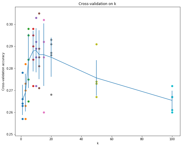
可以看到，第5條豎線對應的均值達到了折線的頂峰，在K_choice裡面第五個K值對應的是K=10，因此best_k的值應該改為10

# Based on the cross-validation results above, choose the best value for k,   
# retrain the classifier using all the training data, and test it on the test
# data. You should be able to get above 28% accuracy on the test data.
best_k = 10

classifier = KNearestNeighbor()
classifier.train(X_train, y_train)
y_test_pred = classifier.predict(X_test, k=best_k)

# Compute and display the accuracy
num_correct = np.sum(y_test_pred == y_test)
accuracy = float(num_correct) / num_test
print ('Got %d / %d correct => accuracy: %f' % (num_correct, num_test, accuracy))

提示說最後的準確率應該比28%大，如果best_k取1時候，執行結果的準確率是27%左右，當把K改為10以後，準確率是：

Got 144 / 500 correct => accuracy: 0.288000

而沒有使用交叉驗證時候，指定K=1和K=5時候的準確率分別為27%和29%（這裡沒弄明白為什麼交叉驗證選出的K=10在測試集上的表現不如動手指定的k=5，可能因為選用的訓練集並不是全部訓練集）

Got 137 / 500 correct => accuracy: 0.274000 #k=1
Got 145 / 500 correct => accuracy: 0.290000 #k=5

2.使用歐式距離計算測試資料和訓練資料的距離矩陣，三種方法，一種使用兩層迴圈，二種使用一層迴圈，最後一種需要用到更多的數學知識和向量化處理，不使用迴圈進行計算：

def compute_distances_two_loops(self, X):
    """
    Compute the distance between each test point in X and each training point
    in self.X_train using a nested loop over both the training data and the 
    test data.

    Inputs:
    - X: A numpy array of shape (num_test, D) containing test data.

    Returns:
    - dists: A numpy array of shape (num_test, num_train) where dists[i, j]
      is the Euclidean distance between the ith test point and the jth training
      point.
    """
    num_test = X.shape[0]
    num_train = self.X_train.shape[0]
    dists = np.zeros((num_test, num_train))
    for i in range(num_test):
      for j in range(num_train):
        #####################################################################
        # TODO:                                                             #
        # Compute the l2 distance between the ith test point and the jth    #
        # training point, and store the result in dists[i, j]. You should   #
        # not use a loop over dimension.                                    #
        #####################################################################
        dists[i,j]=np.sqrt(np.sum(np.square(self.X_train[j,:]-X[i,:])))
        #####################################################################
        #                       END OF YOUR CODE                            #
        #####################################################################
    return dists

  def compute_distances_one_loop(self, X):
    """
    Compute the distance between each test point in X and each training point
    in self.X_train using a single loop over the test data.

    Input / Output: Same as compute_distances_two_loops
    """
    num_test = X.shape[0]
    num_train = self.X_train.shape[0]
    dists = np.zeros((num_test, num_train))
    for i in range(num_test):
      #######################################################################
      # TODO:                                                               #
      # Compute the l2 distance between the ith test point and all training #
      # points, and store the result in dists[i, :].                        #
      #######################################################################
      dists[i,:] = np.sqrt(np.sum(np.square(self.X_train-X[i,:]),axis = 1))
      #np.square是針對每個元素的平方方法
      #######################################################################
      #                         END OF YOUR CODE                            #
      #######################################################################
    return dists

  def compute_distances_no_loops(self, X):
    """
    Compute the distance between each test point in X and each training point
    in self.X_train using no explicit loops.

    Input / Output: Same as compute_distances_two_loops
    """
    num_test = X.shape[0]
    num_train = self.X_train.shape[0]
    dists = np.zeros((num_test, num_train)) 
    #########################################################################
    # TODO:                                                                 #
    # Compute the l2 distance between all test points and all training      #
    # points without using any explicit loops, and store the result in      #
    # dists.                                                                #
    #                                                                       #
    # You should implement this function using only basic array operations; #
    # in particular you should not use functions from scipy.                #
    #                                                                       #
    # HINT: Try to formulate the l2 distance using matrix multiplication    #
    #       and two broadcast sums.                                         #
    #########################################################################
    dists = np.multiply(np.dot(X,self.X_train.T),-2) 
    sq1 = np.sum(np.square(X),axis=1,keepdims = True) 
    sq2 = np.sum(np.square(self.X_train),axis=1) 
    dists = np.add(dists,sq1) 
    dists = np.add(dists,sq2) 
    dists = np.sqrt(dists)
    #########################################################################
    #                         END OF YOUR CODE                              #
    #########################################################################
    return dists

第一種執行的時間效率最低的是使用兩層迴圈，計算每個測試向量和每個訓練向量的向量差，然後使用np.square()計算求得每個元素的平方（也可以使用點乘的方式：np.dot(X[i] - self.X_train[j], X[i] - self.X_train[j])），使用np.sum()計算元素平方的和，最後開方求得的就是該測試向量和訓練向量的歐式距離，所有遍歷下來需要計算500*5000次，也就是測試資料集的行數乘以訓練資料集的行數。

5000行的3072維訓練資料，500行的3072維測試資料，計算的時間花銷是57秒左右：

Two loop version took 57.858908 seconds

第二種方法，使用一層迴圈，遍歷每個測試向量，直接計算每個測試向量(1*3072)和所有訓練向量(5000*3072)的差，得到一個5000*3072的矩陣，然後使用np.square(X)計算每個元素的平方，再使用np.sum(np.square(self.X_train-X[i,:]),axis = 1)計算每行所有列的元素平方的和，再開方得到一個5000*1的向量，以橫向量形式儲存在結果陣列的一行 中，表示的是該測試向量和所有訓練向量的歐式距離，最後得到的就是500*5000的一個結果，也就是測試資料集的行數乘以訓練資料集的行數。

使用一層迴圈的時間開銷是使用兩層迴圈的兩倍，大約106秒：

 One loop version took 106.198080 seconds

最後一種方式不使用迴圈，但是需要用到一點推理歸納：

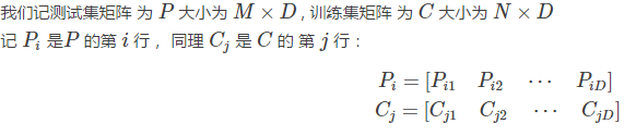
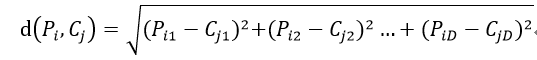
我們先來計算一下 Pi 和 Cj 之間的距離 

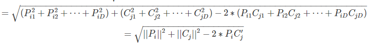
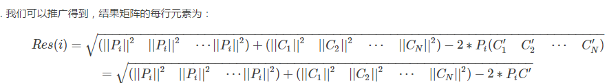
因此，結果矩陣的表示形式為：

換成python程式碼就是:

      dists = np.multiply(np.dot(X,self.X_train.T),-2)  #維度是(500,5000)
    sq1 = np.sum(np.square(X),axis=1,keepdims = True)  #維度是(500,1)
    sq2 = np.sum(np.square(self.X_train),axis=1)     #維度是(5000,)沒有保持維度，也不能保持維度
    dists = np.add(dists,sq1)                  #維度是(500,5000)
    dists = np.add(dists,sq2) 
    dists = np.sqrt(dists)

值得注意的是程式碼中先計算了最後一部分2PC'，此時資料維度是500*5000，然後計算測試資料和訓練資料的元素平方，但是訓練資料不能保持維度，最後使用np.add函式對兩個向量和前面的矩陣進行加法，維度不變，依然是500*5000.