
自然語言處理—文字情感分析
自然語言處理(NLP)中的文字情感分析是一個重要的應用領域,多用於評價性的使用者資訊回饋,如電影影評和購物後的評價。而情感分析主要是通過使用者的回答文字資料(中文),進行文字情感量化分析,現有的情感分析方法:1.情感詞典分析方法。2.機器學習分析方法。
情感詞典分析方法
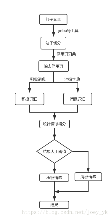
一句話來總結,就是對文字進行切詞,出除掉停用詞,提取出關鍵詞中的積極關鍵詞和消極關鍵詞,計算出情感得分。
先是對文字資料進行切詞,這裡使用中文切詞工具jieba,還有很多其他的切詞工具,如snowNLP等,都有各自的優點,但是切詞越準確得到的結果就越準確。其次就是關於字典的生成,這裡主要是包含三個字典,停用詞字典,積極情感字典,消極情感字典,來源於知網HowNet的字典。停用詞字典包含的是“那麼”,“怎麼”這樣的連線詞還有一些標點符號等,不帶有情感的詞語,將這些詞語去掉後,只剩下了帶有情感的詞語。詞典包含的資料越多,情感預測的也就越準確。
程式碼:
# -*- coding: utf-8 -*-
__author__ = 'JoeyYK'
import jieba
print('loading dictionary dataset...')
#匯入負面情緒字典
negitive_dic = open('negitive_word.txt')
negitive_arr= negitive_dic.readlines()
negitive_word = []
for arr in negitive_arr:
arr = arr.replace("\n", "")
negitive_word.append(arr)
# print(negitive_word) 輸出結果:
/home/joey/anaconda3/bin/python /home/joey/PycharmProjects/workspace/emotion/emotion_test.py
loading dictionary dataset...
Building prefix dict from the default dictionary ...
Loading model from cache /tmp/jieba.cache
以前你們很棒的,現在你們這個維修的進度也太慢了吧,我都等了幾天了,真的是垃圾,太差勁了,我要投訴你們
['以前', '你們', '很棒', '的', ',', '現在', '你們', '這個', '維修', '的', '進度', '也', '太慢', '了', '吧', ',', '我', '都', '等', '了', '幾天', '了', ',', '真的', '是', '垃圾', ',', '太', '差勁', '了', ',', '我要', '投訴', '你們']
['很棒', '維修', '進度', '太慢', '幾天', '真的', '垃圾', '太', '差勁', '我要', '投訴']
Loading model cost 1.298 seconds.
Prefix dict has been built succesfully.
poscount: 1
negcount: 3
final_score: -2

Process finished with exit code 0
詞典法存在很多缺點,詞典法的精確度與詞典的關係非常大,只有詞典的規模足夠大才能並且包含足夠多的該領域的專業資料才能準確的預測情感情況,其次詞典法只是簡單的關鍵詞匹配,數學化的計算出消極和積極詞語的數量來判斷情感是很侷限的,例如“我開始覺得你們非常的差勁,進度慢,效率垃圾,但是我接觸後才發現非常的好”這句話其實表達的是一種讚美的情感可以說是積極的,但是按照詞典法就是不太好的結果。所以我們考慮第二種方法,也就是機器學習方法。
機器學習法
利用機器學習的方法,主要利用的是word2vec這個詞向量模型,將詞轉化成陣列,這樣通過計算詞間的資料距離,來衡量詞之間的相似度,這樣在模型有監督的學習了積極和消極詞向量後,就可以得到結果了。這裡使用的迴圈神經網路LSTM,LSTM的時延效能幫助到詞向量的學習。這裡使用的是tensorflow的深度學習框架。
借用大神程式碼,程式碼地址:https://github.com/vortexJCH/-LSTM-
程式碼:
import warnings
warnings.filterwarnings(action='ignore', category=UserWarning, module='gensim')
import gensim
from gensim.models import word2vec
import jieba
import tensorflow as tf
import numpy as np
import time
from random import shuffle

#----------------------------------
#停用詞獲取
def makeStopWord():
    with open('停用詞.txt','r',encoding = 'utf-8') as f:
        lines = f.readlines()
    stopWord = []
    for line in lines:
        words = jieba.lcut(line,cut_all = False)
        for word in words:
            stopWord.append(word)
    return stopWord

#將詞轉化為陣列
def words2Array(lineList):
    linesArray=[]
    wordsArray=[]
    steps = []
    for line in lineList:
        t = 0
        p = 0
        for i in range(MAX_SIZE):
            if i<len(line):
                try:
                    wordsArray.append(model.wv.word_vec(line[i]))
                    p = p + 1
                except KeyError:
                    t=t+1
                    continue
            else:
               wordsArray.append(np.array([0.0]*dimsh))
        for i in range(t):
            wordsArray.append(np.array([0.0]*dimsh))
        steps.append(p)
        linesArray.append(wordsArray)
        wordsArray = []
    linesArray = np.array(linesArray)
    steps = np.array(steps)
    return linesArray, steps

#將資料轉化為資料
def convert2Data(posArray, negArray, posStep, negStep):
    randIt = []
    data = []
    steps = []
    labels = []
    for i in range(len(posArray)):
        randIt.append([posArray[i], posStep[i], [1,0]])
    for i in range(len(negArray)):
        randIt.append([negArray[i], negStep[i], [0,1]])
    shuffle(randIt)
    for i in range(len(randIt)):
        data.append(randIt[i][0])
        steps.append(randIt[i][1])
        labels.append(randIt[i][2])
    data = np.array(data)
    steps = np.array(steps)
    return data, steps, labels

#獲得檔案中的資料,並且分詞,去除其中的停用詞
def getWords(file):
    wordList = []
    trans = []
    lineList = []
    with open(file,'r',encoding='utf-8') as f:
        lines = f.readlines()
    for line in lines:
        trans = jieba.lcut(line.replace('\n',''), cut_all = False)
        for word in trans:
            if word not in stopWord:
                wordList.append(word)
        lineList.append(wordList)
        wordList = []
    return lineList

#產生訓練資料集和測試資料集
def makeData(posPath,negPath):
    #獲取詞彙,返回型別為[[word1,word2...],[word1,word2...],...]
    pos = getWords(posPath)
    print("The positive data's length is :",len(pos))
    neg = getWords(negPath)
    print("The negative data's length is :",len(neg))
    #將評價資料轉換為矩陣,返回型別為array
    posArray, posSteps = words2Array(pos)
    negArray, negSteps = words2Array(neg)
    #將積極資料和消極資料混合在一起打亂,製作資料集
    Data, Steps, Labels = convert2Data(posArray, negArray, posSteps, negSteps)
    return Data, Steps, Labels


#----------------------------------------------
# Word60.model   60維
# word2vec.model        200維

timeA=time.time()
word2vec_path = 'word2vec/word2vec.model'
model=gensim.models.Word2Vec.load(word2vec_path)
dimsh=model.vector_size
MAX_SIZE=25
stopWord = makeStopWord()

print("In train data:")
trainData, trainSteps, trainLabels = makeData('data/A/Pos-train.txt',
                                              'data/A/Neg-train.txt')
print("In test data:")
testData, testSteps, testLabels = makeData('data/A/Pos-test.txt',
                                           'data/A/Neg-test.txt')
trainLabels = np.array(trainLabels)

del model

# print("-"*30)
# print("The trainData's shape is:",trainData.shape)
# print("The testData's shape is:",testData.shape)
# print("The trainSteps's shape is:",trainSteps.shape)
# print("The testSteps's shape is:",testSteps.shape)
# print("The trainLabels's shape is:",trainLabels.shape)
# print("The testLabels's shape is:",np.array(testLabels).shape)


num_nodes = 128
batch_size = 16
output_size = 2

#使用tensorflow來建立模型
graph = tf.Graph() #定義一個計算圖
with graph.as_default(): #構建計算圖

    tf_train_dataset = tf.placeholder(tf.float32,shape=(batch_size,MAX_SIZE,dimsh))
    tf_train_steps = tf.placeholder(tf.int32,shape=(batch_size))
    tf_train_labels = tf.placeholder(tf.float32,shape=(batch_size,output_size))

    tf_test_dataset = tf.constant(testData,tf.float32)
    tf_test_steps = tf.constant(testSteps,tf.int32)

    #使用LSTM的迴圈神經網路
    lstm_cell = tf.nn.rnn_cell.BasicLSTMCell(num_units = num_nodes,state_is_tuple=True)

    w1 = tf.Variable(tf.truncated_normal([num_nodes,num_nodes // 2], stddev=0.1))
    b1 = tf.Variable(tf.truncated_normal([num_nodes // 2], stddev=0.1))

    w2 = tf.Variable(tf.truncated_normal([num_nodes // 2, 2], stddev=0.1))
    b2 = tf.Variable(tf.truncated_normal([2], stddev=0.1))

    def model(dataset, steps):
        outputs, last_states = tf.nn.dynamic_rnn(cell = lstm_cell,
                                                 dtype = tf.float32,
                                                 sequence_length = steps,
                                                 inputs = dataset)
        hidden = last_states[-1]

        hidden = tf.matmul(hidden, w1) + b1
        logits = tf.matmul(hidden, w2) + b2
        return logits
    train_logits = model(tf_train_dataset, tf_train_steps)
    loss = tf.reduce_mean(
        tf.nn.softmax_cross_entropy_with_logits(labels=tf_train_labels,logits=train_logits))
    optimizer = tf.train.GradientDescentOptimizer(0.01).minimize(loss)
    #預測
    test_prediction = tf.nn.softmax(model(tf_test_dataset, tf_test_steps))

num_steps = 20001
summary_frequency = 500

with tf.Session(graph = graph) as session:
    tf.global_variables_initializer().run()
    print('Initialized')
    mean_loss = 0
    for step in range(num_steps):
        offset = (step * batch_size) % (len(trainLabels)-batch_size)
        feed_dict={tf_train_dataset:trainData[offset:offset + batch_size],
                   tf_train_labels:trainLabels[offset:offset + batch_size],
                   tf_train_steps:trainSteps[offset:offset + batch_size]}
        _, l = session.run([optimizer,loss],
                           feed_dict = feed_dict)
        mean_loss += l
        if step >0 and step % summary_frequency == 0:
            mean_loss = mean_loss / summary_frequency
            print("The step is: %d"%(step))
            print("In train data,the loss is:%.4f"%(mean_loss))
            mean_loss = 0
            acrc = 0
            prediction = session.run(test_prediction)
            for i in range(len(prediction)):
                if prediction[i][testLabels[i].index(1)] > 0.5:
                    acrc = acrc + 1
            print("In test data,the accuracy is:%.2f%%"%((acrc/len(testLabels))*100))
#####################################
timeB=time.time()
print("time cost:",int(timeB-timeA))
結果:
經過20000次的迭代後得到結果
...
The step is: 18000
In train data,the loss is:0.0230
In test data,the accuracy is:97.04%
The step is: 18500
In train data,the loss is:0.0210
In test data,the accuracy is:96.94%
The step is: 19000
In train data,the loss is:0.0180
In test data,the accuracy is:96.89%
The step is: 19500
In train data,the loss is:0.0157
In test data,the accuracy is:97.49%
The step is: 20000
In train data,the loss is:0.0171
In test data,the accuracy is:96.64%
time cost: 809
在語料足夠的情況下,機器學習的方法效果更好一點。