
第4門課程-卷積神經網路-第四周作業(影象風格轉換)
0- 背景
所謂的風格轉換是基於一張Content影象和一張Style影象,將兩者融合,生成一張新的影象,分別兼具兩者的內容和風格。
所需要的依賴如下:
import os
import sys
import scipy.io
import scipy.misc
import matplotlib.pyplot as plt
from matplotlib.pyplot import imshow
from PIL import Image
from nst_utils import *
import numpy as np
import tensorflow as tf

%matplotlib inline
1- Transfer Learning
遷移學習是將其他任務的學習結果應用於一個新的任務。Neural Style Transfer (NST) 就是基於已經訓練過用於其他任務的convolutional network模型。
我們採用的是VGG network,該模型是基於大量的ImageNet database訓練出的,學習到很多高階和低階層次的特徵。
模型載入:
model = load_vgg_model("pretrained-model/imagenet-vgg-verydeep-19.mat")
print(model)
#注:該模型可以從http://www.vlfeat.org/matconvnet/models/beta16/imagenet-vgg-verydeep-19.mat下載到,有些大,500MB左右
輸出資訊:
{'conv5_1': <tf.Tensor 'Relu_12:0' shape=(1, 19, 25, 512) dtype=float32>, 'conv4_1': <tf.Tensor 'Relu_8:0' shape=(1, 38, 50, 512) dtype=float32>, 'avgpool1': <tf.Tensor 'AvgPool:0' shape=(1, 150, 200, 64) dtype=float32>, 'conv4_3': <tf.Tensor 'Relu_10:0' shape=(1, 38, 50, 512) dtype 該model以字典方式儲存,其中的key是變數名,對應的值則是其作為一個tensor所對應的變數值。我們可以通過以下方式將影象輸入到模型中:
model["input"].assign(image)當我們想要檢視特定網路層的啟用值,可以如下操作:
sess.run(model["conv4_2"])conv4_2是對應的Tensor。
2- Neural Style Transfer
構建風格轉換演算法的流程如下:
- 建立content cost function
- 建立the style cost function
- 聯合建立整體代價函式 .
2-1 - Computing the content cost
對於content image C,可以採用以下方式show檢視:
content_image = scipy.misc.imread("images/louvre.jpg")
imshow(content_image)
對於層數的選擇,我們一般不取太大也不取太小。層數太多,提取了更高階特徵,在內容上的相似度,在視覺效果上就不好,層數太少,提取的特徵又太低階,也不行。這點,可以設定不同的網路層數,然後觀察對比具體結果。
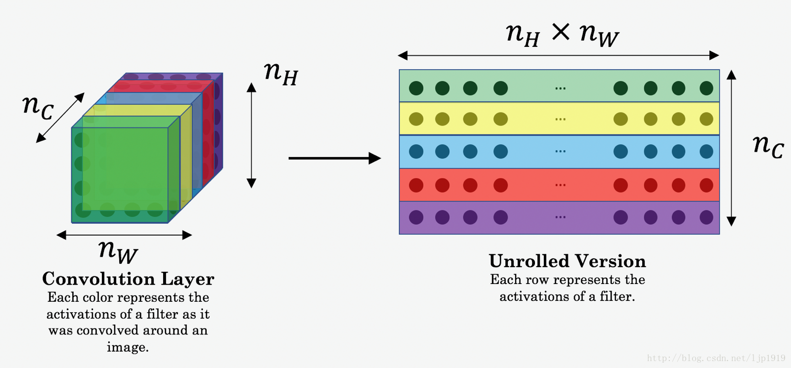
假設我們選取第層的網路進行分析,image C輸入到預訓練的VGG network,並進行前向傳播。 是該層的啟用值,其tensor的尺寸= 。對於image G做相同的處理:影象 G輸入到網路,前向傳播。同樣記 為對應的啟用值。定義content cost function如下:
這裡的 and 都是體資料(volumes ),即三維堆疊起來的。 在計算 cost 時候,可以展開為2D。其實在計算, 可以不用,而在計算style 代價函式時需要。展開方法如下:
content的代價函式實現如下:
# GRADED FUNCTION: compute_content_cost

def compute_content_cost(a_C, a_G):
    """
    Computes the content cost

    Arguments:
    a_C -- tensor of dimension (1, n_H, n_W, n_C), hidden layer activations representing content of the image C
    a_G -- tensor of dimension (1, n_H, n_W, n_C), hidden layer activations representing content of the image G

    Returns:
    J_content -- scalar that you compute using equation 1 above.
    """

    ### START CODE HERE ###
    # Retrieve dimensions from a_G (≈1 line)
    m, n_H, n_W, n_C = a_G.get_shape().as_list()

    # Reshape a_C and a_G (≈2 lines)
    a_C_unrolled = tf.transpose(tf.reshape(a_C, [n_H * n_W, n_C]))
    a_G_unrolled = tf.transpose(tf.reshape(a_G, [n_H * n_W, n_C]))

    # compute the cost with tensorflow (≈1 line)
    J_content = tf.reduce_sum(tf.square(tf.subtract(a_C_unrolled,a_G_unrolled)))/(4*n_H*n_W*n_C)
    ### END CODE HERE ###

    return J_content
測試:
tf.reset_default_graph()

with tf.Session() as test:
    tf.set_random_seed(1)
    a_C = tf.random_normal([1, 4, 4, 3], mean=1, stddev=4)
    a_G = tf.random_normal([1, 4, 4, 3], mean=1, stddev=4)
    J_content = compute_content_cost(a_C, a_G)
    print("J_content = " + str(J_content.eval()))
測試結果:
J_content 6.76559 2-2 Computing the style cost
先看下style影象:
style_image = scipy.misc.imread("images/monet_800600.jpg")
imshow(style_image)
2-2-1 Style matrix
style matrix也稱為”Gram matrix.”(格拉姆矩陣) 。線上性代數中,vectors 的 Gram matrix G 中各個位置的元素是vector中dot product結果,即
Keras卷積神經網路識別CIFAR-10影象(2)
上一篇文章簡單介紹了卷積神經網路的結構,本篇文章則會利用上一篇文章的理論知識搭建神經網路模型來識別CIFAR-10影象。 2.Keras卷積神經網路識別CIFAR-10影象 首先簡單介紹一下什麼是CIFAR-10,CIFAR-10是是用於物件識別的已建立的計算機
使用全卷積神經網路FCN,進行影象語義分割詳解(附程式碼實現)
一.導論 在影象語義分割領域,困擾了電腦科學家很多年的一個問題則是我們如何才能將我們感興趣的物件和不感興趣的物件分別分割開來呢?比如我們有一隻小貓的圖片,怎樣才能夠通過計算機自己對影象進行識別達到將小貓和圖片當中的背景互相分割開來的效果呢?如下圖所示: 而在2015年
Deep Learning.ai學習筆記_第四門課_卷積神經網路
目錄 第一週 卷積神經網路基礎 第二週 深度卷積網路:例項探究 第三週 目標檢測 第四周 特殊應用:人臉識別和神經風格轉換 第一週 卷積神經網路基礎 垂直邊緣檢測器,通過卷積計算,可以把多維矩陣進行降維。如下圖: 卷積運算提供了一個方便的方法來發
卷積神經網路課程筆記-實際應用(第三、四周)
所插入的圖片仍然來源於吳恩達老師的課件。 第三週 目標檢測 1. 物件的分類與定位,在輸出層不僅輸出類別,還應輸出包含物體的邊界框(bx,by,bh,bw),從而達到定位的目的。注意網路的輸出(例如下圖的輸出就有是否為目標,邊界框的引數,以及是哪類的判斷)和損失函式的定義
吳恩達Coursera深度學習課程 deeplearning.ai (4-1) 卷積神經網路--程式設計作業
Part 1:卷積神經網路 本週課程將利用numpy實現卷積層(CONV) 和 池化層(POOL), 包含前向傳播和可選的反向傳播。 變數說明 上標[l][l] 表示神經網路的第幾層 上標(i)(i) 表示第幾個樣本 上標[i][i] 表示第幾個mi
吳恩達Coursera深度學習課程 deeplearning.ai (4-1) 卷積神經網路--課程筆記
本課主要講解了卷積神經網路的基礎知識,包括卷積層基礎(卷積核、Padding、Stride),卷積神經網路的基礎:卷積層、池化層、全連線層。 主要知識點 卷積核: 過濾器,各元素相乘再相加 nxn * fxf -> (n-f+1)x(n-f+1)
DeepLearning.ai作業:(4-1)-- 卷積神經網路(Foundations of CNN)
title: ‘DeepLearning.ai作業:(4-1)-- 卷積神經網路(Foundations of CNN)’ id: dl-ai-4-1h tags: dl.ai homework categories: AI Deep Learning d
DeepLearning.ai筆記:(4-1)-- 卷積神經網路(Foundations of CNN)
title: ‘DeepLearning.ai筆記:(4-1)-- 卷積神經網路(Foundations of CNN)’ id: dl-ai-4-1 tags: dl.ai categories: AI Deep Learning date: 2018-09-
卷積神經網路(4)----目標檢測
一、分類、定位和檢測 簡單來說,分類、定位和檢測的區別如下: 分類:是什麼? 定位:在哪裡?是什麼?(單個目標) 檢測:在哪裡?分別是什麼?(多個目標) (1)目標分