
MATLAB學習筆記 學習總結歸納(第一週)
此學習總結歸納為自己在這一週學習知識的總結,進行歸納整理,如有錯誤,請批評指正
本文進度-第1章~第3章
效能測試
時間
tic toc 用於記錄所包含的語句的執行時間
tic; function(); toc % 返回函式執行時間timeit(function) 用於記錄傳入的函式控制代碼的執行時間
f = @() function(x); % 函式控制代碼
timeit(f) % 返回函式執行時間(不是很準確,此函式中有一些檢測函式執行情況的函式,佔用一部分時間,不過用起來很方便)
物件操作
矩陣
eye(n, m) 產生單位矩陣(生成n*m的單位矩陣)
f = eye(2)
f = eye(1, 2)
zeros(x, y, z) 生成x*y*z的三維矩陣(個數無限制)每個元素都為0
f = zeros(1, 2, 3);
f = zeros(1);
ones(x, y, z) 生成x*y*z的三維矩陣(個數無限制)每個元素都為1
f = ones(1, 2, 3);linspace(a, b, numel(T)) 線性插值(相當於建立一個行向量,其每個元素的值為a~b的線性值-斜率為1)
linspace(1, 0, 25)meshgrid(x, y, z) 用於生成二維、三維陣列(速度快,我的電腦的話,比正常的forforfor快5-10倍)
以二維為例,C返回一個二維陣列,一共有numel(x)列,numel(y)行,每行數字相同,每列對應為x[id],R 則與之相反。
[C, R] = meshgrid(1:2:10, 1:3:30);prod(A, n) 返回傳入引數的乘積 (預設n為1[不寫即為1])
此函式有3種常用情況
* 當傳入引數為一維陣列(只有一行/一列)時,傳出為元素的乘積
prod([1 2 3 4 5]) % 返回 120當傳入引數為二維陣列時,傳出為每列的乘積
prod([1 2;3 4]) % 返回3 8當傳入引數為一個二維陣列和一個數(代表維度),則會返回以這個維度為基準的每維的乘積
prod([1 2; 3 4], 2) % 返回 2 12padarray(A, [x, y], method, direction) 填充陣列,第一個引數為要填充的陣列,x表示在x軸,要填充幾個,y表示在y軸要填充幾個,method(方法)有四種情況(書上有三種- -),direction(方向)也有三種情況
方法: P ‘replicate’ ‘symmetric’ ‘circular’
方向: ‘pre’ ‘post’ ‘both’
padarray([1 2; 3 4], [3 2], 'post')
padarray([1 2; 3 4], [3 2], 'pre')
padarray([1 2; 3 4], [3 2], 'both')
padarray([1 2; 3 4], [3 2], 5, 'post')
padarray([1 2; 3 4], [3 2], 5, 'pre')
padarray([1 2; 3 4], [3 2], 5, 'both')
padarray([1 2; 3 4], [3 2], 'replicate', 'post')
padarray([1 2; 3 4], [3 2], 'replicate', 'pre')
padarray([1 2; 3 4], [3 2], 'replicate', 'both')
padarray([1 2; 3 4], [3 2], 'symmetric', 'post')
padarray([1 2; 3 4], [3 2], 'symmetric', 'pre')
padarray([1 2; 3 4], [3 2], 'symmetric', 'both')
padarray([1 2; 3 4], [3 2], 'circular', 'post')
padarray([1 2; 3 4], [3 2], 'circular', 'pre')
padarray([1 2; 3 4], [3 2], 'circular', 'both')
symmetric 就是映象複製, replicate就是直接複製邊界, circular就是週期複製,post就是在每個維度後面填充, pre就是在前面, both就是post+pre。
size(A, n) 返回A矩陣的第n維有幾個,預設為全部(三維則返回三個)
f = zeros(1, 2, 3);
size(f)
size(f, 1)
% size(f, 0) % 會報錯,因為維度從1開始(不像程式語言)
numel(A) 返回A矩陣的元素個數(全部元素,跨維度計數)
f = zeros(1, 2, 3);
numel(f)
ndims(A) 返回矩陣是幾維.
A = ones(1, 2, 3);
ndims(A) % 返回3
影象
imread(fileName) 讀取名為fileName的圖片,範圍型別根據圖片不同而不同
f = imread('coins.png');imwrite(image, fileName) 將圖片image, 儲存為fileName
fileName可以包含路徑(相對、絕對都可以),格式根據給定格式,函式會自動轉換
f = imread('coins.png');
imwrite(f, '1.jpg');
imwrite(f, 'c:\1.png');
imfinfo(fileName) 將fileName的圖片資訊讀出來
f = imfinfo('conins.png')顯示圖片 imshow(image) 將圖片顯示(在上一個視窗顯示,如果沒有則新建一個)
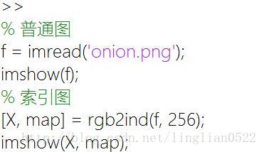
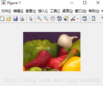
% 普通圖
f = imread('onion.png');
imshow(f);
% 索引圖
[X, map] = rgb2ind(f, 256);
imshow(X, map);- 輸入:
- 輸出:
影象轉換
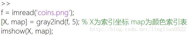
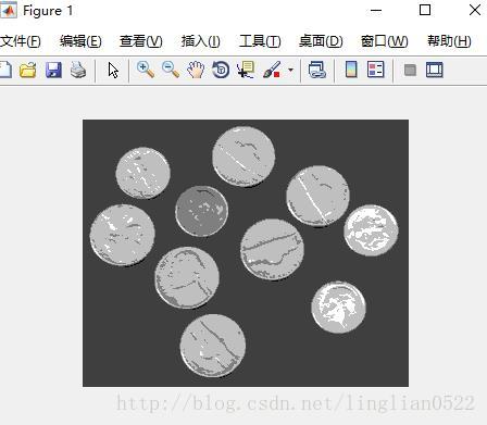
gray2ind(iamge, n) 將傳入的灰度圖轉化索引圖, n代表要分為幾個索引顏色
f = imread('coins.png');
[X, map] = gray2ind(f, 5); % X為索引座標 map為顏色索引表
imshow(X, map);- 輸入:
- 輸出:
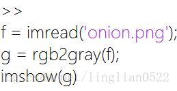
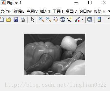
rgb2gray(image) 將rgb轉為gray(灰度圖)
f = imread('onion.png');
g = rgb2gray(f);
imshow(g)- 輸入:
- 輸出:
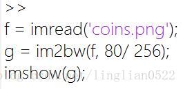
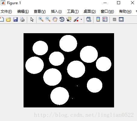
im2bw(image, level) 將圖轉換為二值圖,level為閾值(區間為[0, 1])
低於level 都為黑色(0), 否則為白色(1)
f = imread('coins.png');
g = im2bw(f, 80/ 256);
imshow(g);- 輸入:
- 輸出:
ind2gray(X, map) 從索引圖到灰度圖
ind2rgb(X, map) 從索引圖到RGB圖
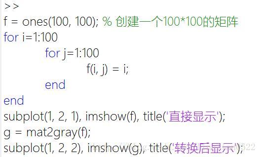
**mat2gray() 將矩陣轉化為灰度圖
f = ones(100, 100); % 建立一個100*100的矩陣
for i=1:100
    for j=1:100
        f(i, j) = i;
    end
end
subplot(1, 2, 1), imshow(f), title('直接顯示');
g = mat2gray(f);
subplot(1, 2, 2), imshow(g), title('轉換後顯示');- 輸入:
- 輸出:
影象處理
直方圖
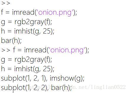
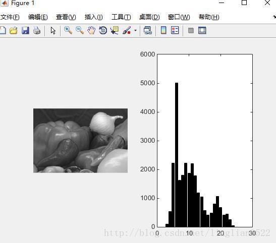
imhist(image, num) 歸一化直方圖
image 表示要處理的圖
num表示將灰度級分為平等的幾份
返回的則是灰度範圍在每份灰度級中的畫素個數
f = imread('onion.png');
g = rgb2gray(f);
h = imhist(g, 25);
subplot(1, 2, 1), imshow(g);
subplot(1, 2, 2), bar(h);- 輸入:
- 輸出:
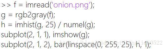
bar(horz, z, width) 繪製條形圖
horz 表示 水平增量,需要與z的行數相同。
z 表示要顯示的條形圖的資料
width 表示條形圖的寬度
f = imread('onion.png');
g = rgb2gray(f);
h = imhist(g, 25) / numel(g);
subplot(2, 1, 1), imshow(g);
subplot(2, 1, 2), bar(linspace(0, 255, 25), h, 1);- 輸入:
- 輸出:
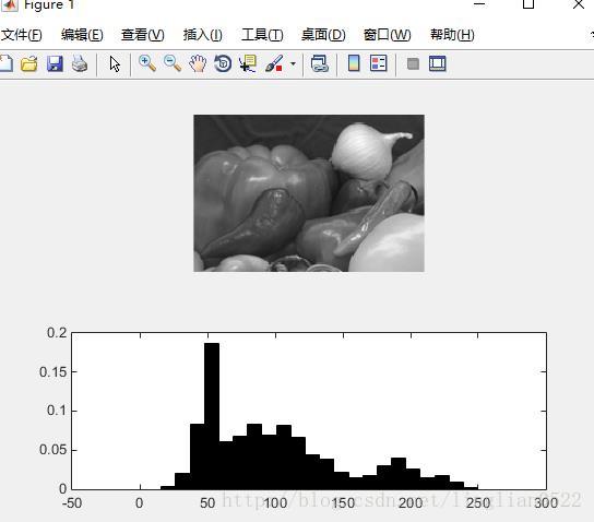
stem(z) 生成一個桿狀圖(也可以省略h)
f = imread('onion.png');
g = rgb2gray(f);
h = imhist(g, 25) / numel(g);
subplot(1, 2, 1), stem(h);
subplot(1, 2, 2), stem(linspace(0, 1, 25), h);- 輸入:
- 輸出:
stem 還有一個引數,表示桿狀圖以什麼形式顯示
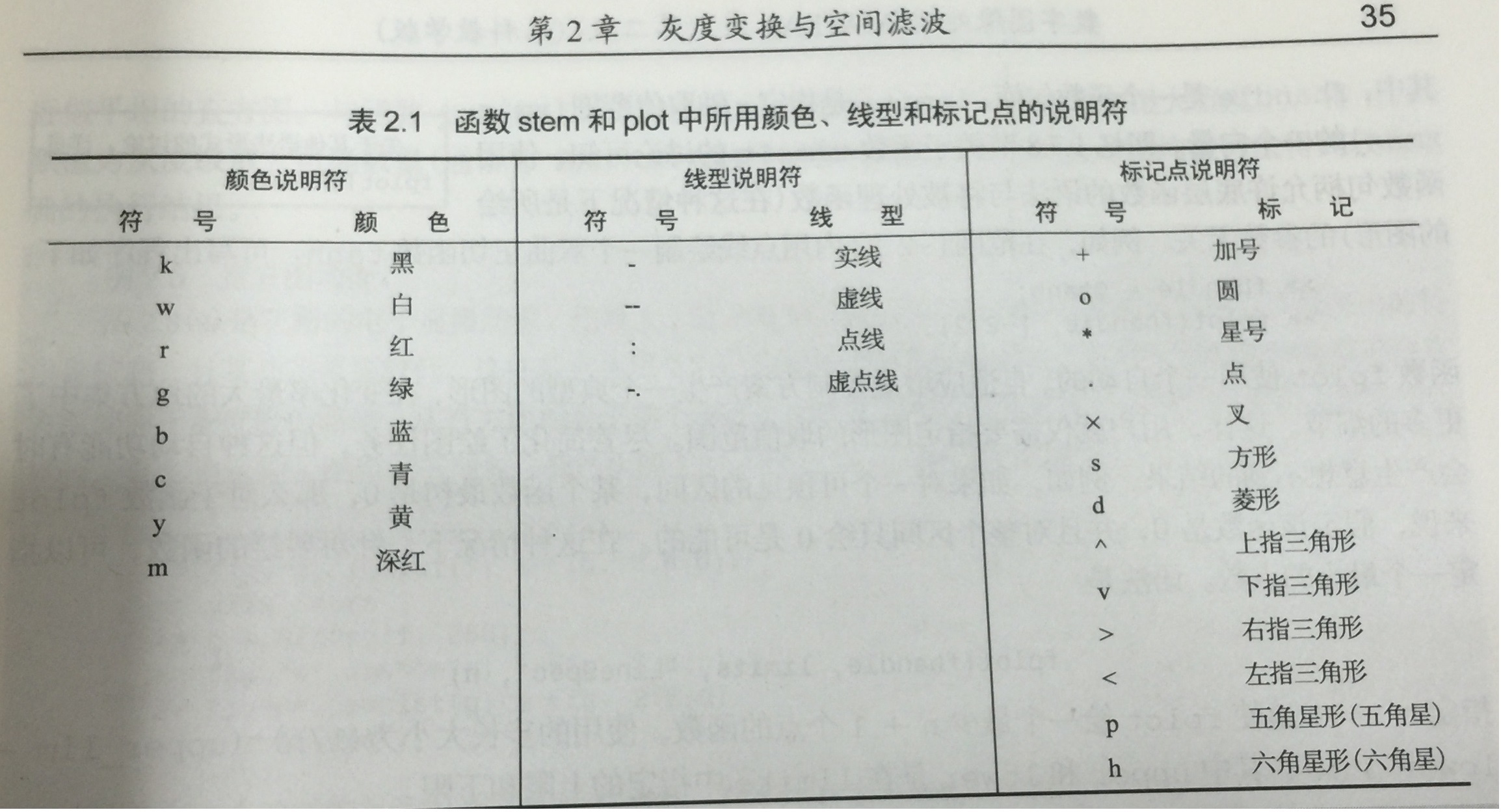
stem(h, 'k:p')具體如下
‘顏色說明符+線型說明符+標記點說明符’
plot 生成一個折線圖,用法跟stem一樣
f = imread('onion.png');
g = rgb2gray(f);
h = imhist(g, 25) / numel(g);
subplot(1, 2, 1), plot (h);
subplot(1, 2, 2), plot (linspace(0, 1, 25), h);
axis([xMin xMax yMin yMax]) 設定上面最近顯示的圖表的x軸和y軸的範圍
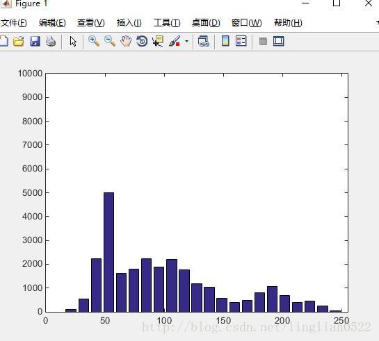
f = imread('onion.png');
g = rgb2gray(f);
h = imhist(g, 25);
z = linspace(0, 255, 25);
bar(z, h)
axis([0 255 0 10000])- 輸入:
- 輸出
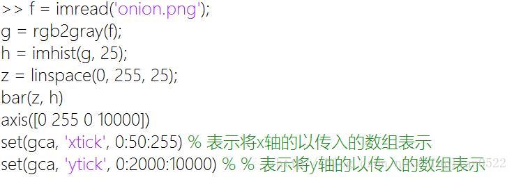
接著下面可以跟著二行
set(gca, ‘xtick’, 0:50:255) % 表示將x軸的以傳入的陣列表示
set(gca, ‘ytick’, 0:2000:10000) % % 表示將y軸的以傳入的陣列表示
* 輸入:
* 輸出
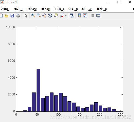
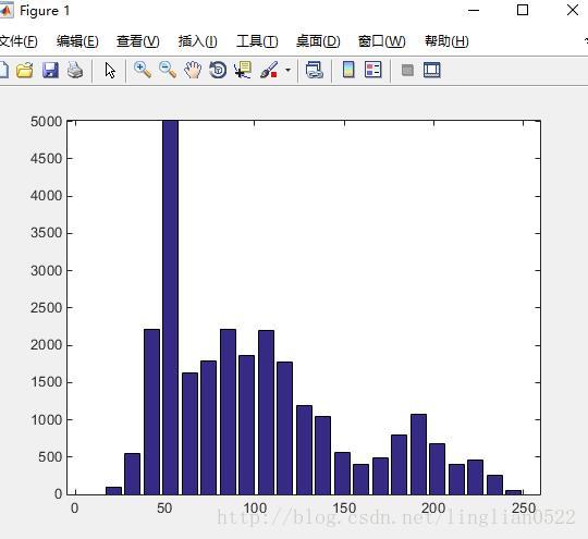
axis tight 自適應圖示
f = imread('onion.png');
g = rgb2gray(f);
h = imhist(g, 25);
z = linspace(0, 255, 25);
bar(z, h)
axis tight- 輸入:
- 輸出:
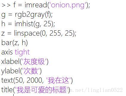
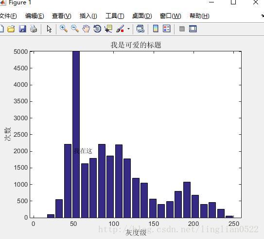
xlabel ylabel 給x和y軸新增標記
xlabel('灰度級')
ylabel('次數')
text(x, y, text) 在x軸的值為x,y軸的值為y處新增text檔案
text(50, 2000, '50,2000')title(title) 給圖片新增標題
title('我是可愛的標題')- 輸入:
- 輸出:
hold on, hold off 開啟、關閉保持當前圖示狀態
bar(z, h)
hold on
stem(z, h)
hold off
bar(z, h)
ylim xlim 設定y軸x軸的範圍(預設就是auto狀態)
ylim([0 60000])
xlim([0 255])
灰度級
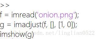
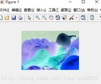
imadjust(image, [low_in high_in], [low_out high_out], gamma) 用於將影象進行灰度級轉換
f = imread('onion.png');
g = imadjust(f, [], [1, 0]);
imshow(g)
imcomplement(image) 獲得圖片的負片, 可以實現CMY模型與RGB互換
rgb = imcomplement(cmy);
cmy = imcomplement(rgb);
上面二個結果一樣
* 輸入:
* 輸出:
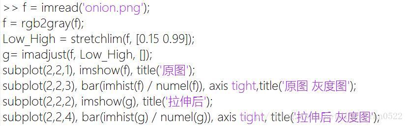
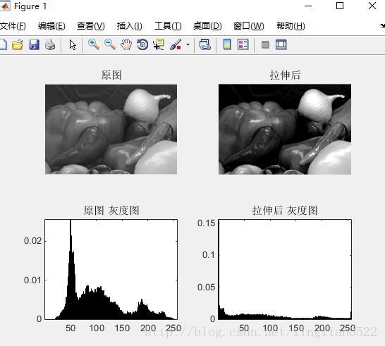
stretchlim(image, tol) 用於實現對比度拉伸
f = imread('onion.png');
f = rgb2gray(f);
Low_High = stretchlim(f, [0.15 0.99]);
g= imadjust(f, Low_High, []);
subplot(2,2,1), imshow(f), title('原圖');
subplot(2,2,3), bar(imhist(f) / numel(f)), axis tight,title('原圖 灰度圖');
subplot(2,2,2), imshow(g), title('拉伸後');
subplot(2,2,4), bar(imhist(g) / numel(g)), axis tight, title('拉伸後 灰度圖');- 輸入:
- 輸出:
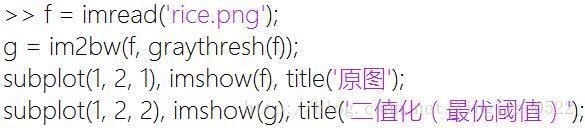
graythresh(image) 獲得圖片最優的閾值。
f = imread('rice.png');
g = im2bw(f, graythresh(f));
subplot(1, 2, 1), imshow(f), title('原圖');
subplot(1, 2, 2), imshow(g), title('二值化(最優閾值)');- 輸入:
- 輸出:

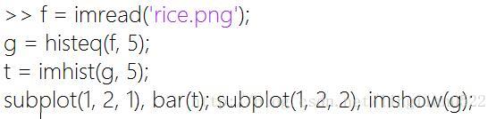
histeq(image, num) 該函式可以將輸入的圖片按灰度級分為num份,使得每份所佔的比例近似相等。
f = imread('rice.png');
g = histeq(f, 5);
t = imhist(g, 5);
subplot(1, 2, 1), bar(t); subplot(1, 2, 2), imshow(g);- 輸入:
- 輸出:
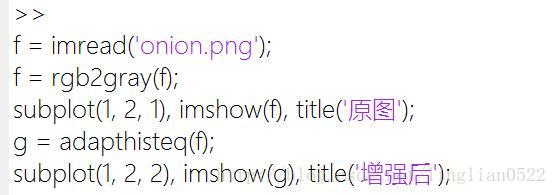
adapthisteq(image) 將影象對比度增強
f = imread('onion.png');
f = rgb2gray(f);
subplot(1, 2, 1), imshow(f), title('原圖');
g = adapthisteq(f);
subplot(1, 2, 2), imshow(g), title('增強後');- 輸入:
- 輸出:
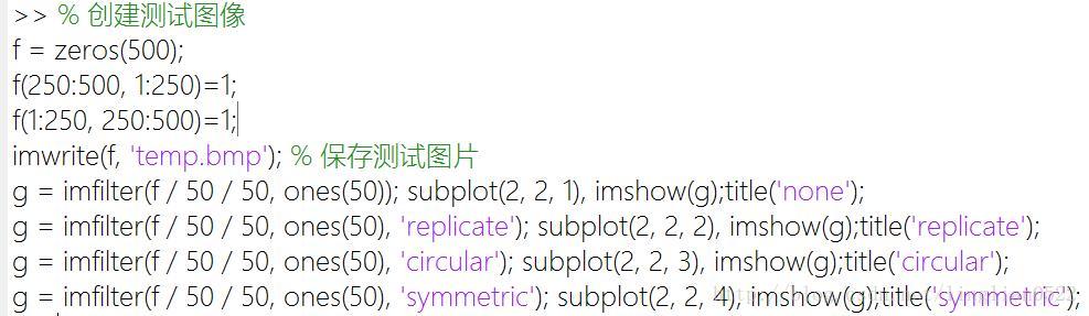
imfilter(image, mod) 線性濾波
可選引數為三個,分別是濾波模式、邊界選項、大小選項
濾波模式: ‘corr’ ‘conv’
邊界選項: P ‘replicate’ ‘symmetric’ ‘circular’
大小選項: ‘full’ ‘same’
% 建立測試影象
f = zeros(500);
f(250:500, 1:250)=1;
f(1:250, 250:500)=1;
imwrite(f, 'temp.bmp'); % 儲存測試圖片
g = imfilter(f / 50 / 50, ones(50)); subplot(2, 2, 1), imshow(g);title('none');
g = imfilter(f / 50 / 50, ones(50), 'replicate'); subplot(2, 2, 2), imshow(g);title('replicate');
g = imfilter(f / 50 / 50, ones(50), 'circular'); subplot(2, 2, 3), imshow(g);title('circular');
g = imfilter(f / 50 / 50, ones(50), 'symmetric'); subplot(2, 2, 4), imshow(g);title('symmetric');- 輸入:
- 輸出:
colfilt(image, [m n], ‘sliding’, fun) 非線性空間濾波, 傳入圖片,濾波區域,和函式控制代碼
t = colfilt(g, [5 5], 'sliding', fun);
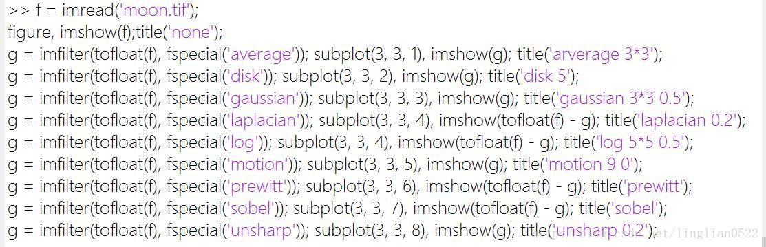
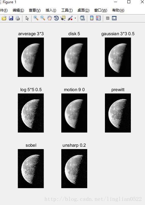
t = gscale(t, 'full16'); % 該函式看附錄fspecial(type, paramters) 線性空間濾波器,type值有9種情況,對應paramters也不同
type : ‘average’ ‘disk’ ‘gaussian’ ‘laplacian’ ‘log’ ‘motion’ ‘prewitt’ ‘sobel’ ‘unsharp’
paramters: [r c] r [r c], sig alpha [r c], sig len, theta null null alpha (與上面的一一對應,null為沒有)
f = imread('moon.tif');
figure, imshow(f);title('none');
g = imfilter(tofloat(f), fspecial('average')); subplot(3, 3, 1), imshow(g); title('arverage 3*3');
g = imfilter(tofloat(f), fspecial('disk')); subplot(3, 3, 2), imshow(g); title('disk 5');
g = imfilter(tofloat(f), fspecial('gaussian')); subplot(3, 3, 3), imshow(g); title('gaussian 3*3 0.5');
g = imfilter(tofloat(f), fspecial('laplacian')); subplot(3, 3, 4), imshow(tofloat(f) - g); title('laplacian 0.2');
g = imfilter(tofloat(f), fspecial('log')); subplot(3, 3, 4), imshow(tofloat(f) - g); title('log 5*5 0.5');
g = imfilter(tofloat(f), fspecial('motion')); subplot(3, 3, 5), imshow(g); title('motion 9 0');
g = imfilter(tofloat(f), fspecial('prewitt')); subplot(3, 3, 6), imshow(tofloat(f) - g); title('prewitt');
g = imfilter(tofloat(f), fspecial('sobel')); subplot(3, 3, 7), imshow(tofloat(f) - g); title('sobel');
g = imfilter(tofloat(f), fspecial('unsharp')); subplot(3, 3, 8), imshow(g); title('unsharp 0.2');
引數的具體定義直接輸入 doc fspecial 即可
* 輸入:
* 輸出:
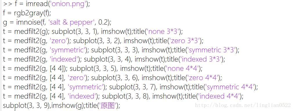
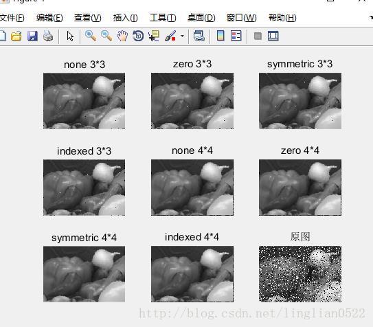
medfilt2(image, [x y], padpot) 非線性濾波器 [x y]預設為3*3表示濾波區域, padpot表示濾波方式,分為三種
padpot: ‘zero’ ‘symmetric’ ‘indexed’
f = imread('onion.png');
f = rgb2gray(f);
g = imnoise(f, 'salt & pepper', 0.2);
t = medfilt2(g); subplot(3, 3, 1), imshow(t);title('none 3*3');
t = medfilt2(g, 'zero'); subplot(3, 3, 2), imshow(t);title('zero 3*3');
t = medfilt2(g, 'symmetric'); subplot(3, 3, 3), imshow(t);title('symmetric 3*3');
t = medfilt2(g, 'indexed'); subplot(3, 3, 4), imshow(t);title('indexed 3*3');
t = medfilt2(g, [4 4]); subplot(3, 3, 5), imshow(t);title('none 4*4');
t = medfilt2(g, [4 4], 'zero'); subplot(3, 3, 6), imshow(t);title('zero 4*4');
t = medfilt2(g, [4 4], 'symmetric'); subplot(3, 3, 7), imshow(t);title('symmetric 4*4');
t = medfilt2(g, [4 4], 'indexed'); subplot(3, 3, 8), imshow(t);title('indexed 4*4');
subplot(3, 3, 9),imshow(g);title('原圖');
去燥效果明顯,但是具體引數的話,還是看出來太大的差別(濾波區域的設定還是很重要地)。
* 輸入:
* 輸出:
輸入輸出
視窗
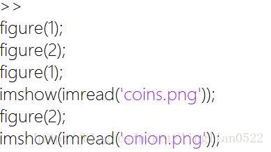
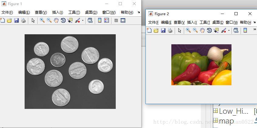
figure(h) 開啟一個新視窗(將h視窗置頂,h省略時則新建一個視窗)
figure(1);
figure(2);
figure(1);
imshow(imread('coins.png'));
figure(2);
imshow(imread('onion.png'));- 輸入:
- 輸出:
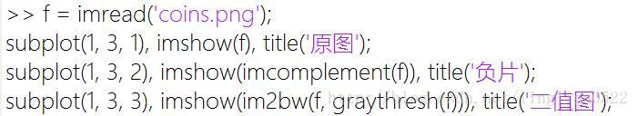
subplot(h, w, id) 將最近顯示的的視窗(之前沒有顯示的話,會新建一個視窗),分為高位h, 寬為w個單位,並指定下一個要顯示的影象在這個視窗的第id個單位格;
f = imread('coins.png');
subplot(1, 3, 1), imshow(f), title('原圖');
subplot(1, 3, 2), imshow(imcomplement(f)), title('負片');
subplot(1, 3, 3), imshow(im2bw(f, graythresh(f))), title('二值圖');- 輸入:
- 輸出:

控制檯
disp 顯示資訊
disp 'Asdasd' % 輸出Asdasdinput 從鍵盤中輸入
t = input('asd', 's'); % 引數s表示將結果以字串的形式儲存error 顯示警告
error '這是錯誤的!' % 這裡是紅色警告字附錄
預設圖片
函式
gscale.m
function g = gscale(f, varargin)
if isempty(varargin)
    method = 'full8';
else
    method = varargin{1};
end

if strcmp(class(f), 'double') && (max(f(:)) > 1 || min(f(:)) < 0)
    f = mat2gray(f);
end

switch method
    case 'full8'
        g = im2uint8(mat2gray(double(f)));
    case 'full16'
        g = im2uint16(mat2gray(double(f)));
    case 'minmax'
        low = varargin{2};
        high = varargin{3};
        if low > 1 || low < 0 || high > 1 || high < 0
            error('low | high must be [0, 1]');
        end
        if strcmp(class(f), 'double')
            low_in = max(f(:));
            high_in = max(f(:));
        elseif strcmp(class(f), 'uint8')
            low_in = double(min(f(:))) ./ 255;
            high_in = double(max(f(:))) ./ 255;
        elseif strcmp(class(f), 'uint16')
            low_in = double(min(f(:))) ./ 65535;
            high_in = double(max(f(:))) ./ 65535;
        end
        g = imadjust(f, [low_in high_in], [low high]);

    otherwise
        error('Unknow method');
end
tofloat.m
function [out, revertclass] = tofloat(in)
identity = @(x) x;
tosingle = @im2single;
table = {'uint8', tosingle, @im2uint8
    'uint16', tosingle, @im2uint16
    'uint32', tosingle, @im2int32
    'logical', tosingle, @logical
    'double', identity, identity
    'single', identity, identity};

classIndex = find(strcmp(class(in), table(:, 1)));
if isempty(classIndex)
    error('Unsupported input image class');
end

out = table{classIndex, 2}(in);

revertclass = table{classIndex, 3};