
TensorFlow的邏輯迴歸實現
阿新 • • 發佈:2019-01-09

開啟微信掃一掃,關注微信公眾號【資料與演算法聯盟】
轉載請註明出處:http://blog.csdn.net/gamer_gyt
博主微博:http://weibo.com/234654758
Github:https://github.com/thinkgamer
邏輯迴歸我們都知道是用來進行二分類處理的,裡邊經常用到的階躍函式是海維塞得階躍函式(Sigmoid函式)。
邏輯迴歸簡介
線性迴歸能對連續值結果進行預測,而現實生活中常見的另外一類問題是,分類問題。最簡單的情況是是與否的二分類問題。比如說醫生需要判斷病人是否生病,銀行要判斷一個人的信用程度是否達到可以給他發信用卡的程度,郵件收件箱要自動對郵件分類為正常郵件和垃圾郵件等等。
當然,我們最直接的想法是,既然能夠用線性迴歸預測出連續值結果,那根據結果設定一個閾值是不是就可以解決這個問題了呢?然後在大多數情況下需要學習的分類資料並沒有那麼精準,這個時候閾值的設定就沒卵用了,這時候就需要邏輯迴歸了,邏輯迴歸的核心思想就是通過對線性迴歸的計算結果進行一個對映,使之輸出的結果為0~1之間的概率值。
這個時候就需要一個單位階躍函式,常使用的就是Sigmoid函式。

求導之後為:
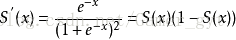
對應的影象為:

關於Softmax Regression
TF中基於LR的多分類實現
# coding: utf-8
'''
create by: Thinkgamer
create time: 2018/04/22
desc: 使用tensorflow建立邏輯迴歸模型 ,分類
''' # 載入mnist資料集
from tensorflow.examples.tutorials.mnist import input_data
print("load finish")
mnist = input_data.read_data_sets("MNIST_data/",one_hot=True)
print(type(mnist))
train_img = mnist.train.images
train_label = mnist.train 輸出為:
load finish
Extracting MNIST_data/train-images-idx3-ubyte.gz
Extracting MNIST_data/train-labels-idx1-ubyte.gz
Extracting MNIST_data/t10k-images-idx3-ubyte.gz
Extracting MNIST_data/t10k-labels-idx1-ubyte.gz
<class 'tensorflow.contrib.learn.python.learn.datasets.base.Datasets'>
訓練集型別: <class 'numpy.ndarray'>
訓練集維度: (55000, 784)
測試集型別: <class 'numpy.ndarray'>
測試集維度: (10000, 784)
[0. 0. 0. 0. 0. 0. 0. 1. 0. 0.]
x = tf.placeholder("float",[None,784])
y = tf.placeholder("float",[None,10])
W = tf.Variable(tf.zeros([784,10])) # 表示權重,784個維度,10種類別
b = tf.Variable(tf.zeros([10])) # 表示 是10分類,這裡選用0值初始化,一般採用高斯初始化
# 表示預測值結果
actv = tf.nn.softmax(tf.matmul(x,W)+b)
# 構造損失函式
# 損失函式 -log p, 各個維度損失函式求和之後,求均值
cost= tf.reduce_mean(-tf.reduce_sum(y*tf.log(actv),reduction_indices=1))
# Optimizer 指定優化器 梯度下降
learning_rate = 0.1
optm = tf.train.GradientDescentOptimizer(learning_rate=learning_rate).minimize(cost)sess = tf.InteractiveSession()
# 函式學習 tf.argmax 返回最大值的索引
arr = np.array([
[1,2,3,4,5],
[6,7,8,9,10]
])
print(tf.shape(arr).eval())
print(tf.argmax(arr,0).eval()) #eval(session=sess)) 0 是按列 1 是按行
print(tf.argmax(arr,1).eval()) # 預測
pred = tf.equal(tf.argmax(actv,1),tf.argmax(y,1))
# 準確率
accr = tf.reduce_mean(tf.cast(pred,"float"))
# init
init = tf.global_variables_initializer()training_epochs = 50 # 樣本迭代次數
batch_size = 100 # 每次迭代使用的樣本
display_step = 50
sess = tf.Session()
sess.run(init)
# MINI-BATCH LEARENING
for epoch in range(training_epochs):
avg_cost = 0.
number_batch = int(mnist.train.num_examples/batch_size)
for i in range(number_batch):
batch_xs,batch_ys = mnist.train.next_batch(batch_size)
sess.run(optm,feed_dict={x:batch_xs,y:batch_ys})
feeds = {x: batch_xs,y: batch_ys}
avg_cost += sess.run(cost,feed_dict=feeds)/number_batch
# DISPLAY
if epoch % display_step ==0 :
feeds_train = {x:batch_xs,y:batch_ys}
feeds_test = {x: mnist.test.images,y:mnist.test.labels}
train_acc = sess.run(accr,feed_dict=feeds_train)
test_acc = sess.run(accr,feed_dict=feeds_test)
print(("Epoch: %03d/%03d cost:%.9f train_acc: %.3f test_acc: %.3f") % (epoch,training_epochs,avg_cost,train_acc,test_acc))
print("Done")
開啟微信掃一掃,加入資料與演算法交流大群