
特徵臉是怎麼提取的之主成分分析法PCA
機器學習筆記 多項式迴歸這一篇中,我們講到了如何構造新的特徵,相當於對樣本資料進行升維.
那麼相應的,我們肯定有資料的降維.那麼現在思考兩個問題
- 為什麼需要降維
- 為什麼可以降維
第一個問題很好理解,假設我們用KNN訓練一些樣本資料,相比於有1W個特徵的樣本,肯定是訓練有1K個特徵的樣本速度更快,因為計算量更小嘛.
第二個問題,為什麼可以降維.一個樣本原先有1W個特徵,現在減少到1K個,不管如何變換,資料包含的資訊肯定是減少了,這是毫無疑問的.但是資訊的減少是否意味著我們對於樣本的認知能力的下降?這個則未必.
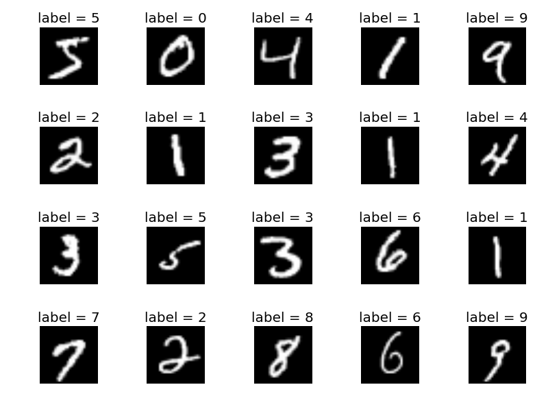
以minist資料集為例,每一個數字圖片都由N個畫素構成,即樣本有N個特徵,但是我們不需要精確地知道每一個畫素的值,依然能夠分辨出這個數字是幾,你可以通俗地理解為,比如你把每張圖的邊邊角角都減掉,並不影響你識別這是幾。 由此,我們知道,樣本特徵的重要性並不是一致的,有的重要,也即所謂的主成分.
現在問題則轉換為:我們怎麼樣尋找到一種方法,使得降維後"重要的特徵"儘可能地保留,也即降維後資訊的丟失最少?
依然從一個極端的例子入手,假設我們有M個樣本,每個樣本2個特徵,特徵1的波動幅度很大,特徵2的波動幅度很小.

此時,如果要把這M個樣本降成1維,採用最簡單粗暴的方式,丟棄一個特徵,是丟棄feature1呢還是feature2呢?
如果,丟棄feature1的話,我們的樣本就只剩下了feature2,而feature2的值在3附近微小的波動,幾乎沒有變化. 沒有變化,機器學習演算法就沒法從中學習到足夠的資訊.比如M個樣本對應著M個label,這M個label各不相同.來了個新樣本,特徵值還是3,這時候我們是沒法推算出新樣本的label的.
對機器學習演算法而言,我們希望在合理的範圍內,資料的分佈越分散越好,即資料的方差越大越好,這樣才能學習到足夠多的資訊.
而這也正是PCA降維的理論基礎:我們希望找到一個新的N維座標系,使得資料在這個新的N維座標系的前K個座標軸上分佈,方差最大.這樣的N維座標系中的K個座標軸就是我們所要尋找的K個主成分.
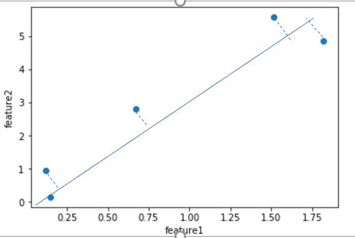
比如對這個圖中的藍色的點而言,我們希望找到一個向量w(圖中的藍色線),使得各點在w上的投影點,方差最大.樣本點$X^{(i)}$投影到單位向量w後得到$X_p^{(i)}$,這些新的樣本點的方差為$\frac{\sum_{i=1}^m (X_p^{(i)} - \overline X_p)^2)} m$,為了方便計算,在向w投影之前,我們對樣本X做demean去均值處理,即每個特徵值減去該維度特徵的均值,這個操作並不會影響資料的分佈.demean後的樣本點投影到w後得到的新樣本點的方差變為$\frac{\sum_{i=1}^m (X_p^{(i)})^2)} m$.注意這裡$X_p^{(i)}$是一個向量.所以我們的方差可以轉變為$$Var(X_p) = \frac{\sum_{i=1}^m || X_p^{(i)} ||^2)} m$$

注意,樣本點$X^{(i)}$投影到單位向量w後得到$X_p^{(i)}$,由向量點乘的定義我們能夠得到$X^{(i)} \cdot w = || X^{(i)}|| \cdot || w|| \cdot \cos \theta = || X^{(i)}|| \cdot \cos \theta = || X_p^{(i)} ||$.由此我們的目標轉變為使得$$Var(X_p) = \frac{\sum_{i=1}^m X^{(i)} \cdot w^2)} m$$最大化.
接下來我們用梯度上升法求出這個w。現在先不用管梯度上升法是怎麼回事,本篇重點在於理解PCA。梯度下降法梯度上升法以後會再寫博文解釋.這個w也就是我們的第一主成分.即樣本投影到這個方向後,方差最大,損失資訊最少.那麼現在我們如何求出第二主成分呢?
求出這個w之後,注意w是一個N維向量. 我們就可以得到X在w之外剩餘的分量為$X^{’(i)}=X^{(i)}-X_p^{(i)}=X^{(i)}-X^{(i) \cdot w}$,對$X^{’(i)}$,我們再次求出一個w2,使得其在w2上的投影的方差最大,求解方法同上.
我們不斷迴圈這個過程,就可以求解出k個w,記做
$$W_k=\begin{bmatrix} W_1^{(1)}& W_2^{(1)}& … &W_n^{(1)} \\ W_1^{(2)}& W_2^{(2)}& … &W_n^{(2)} \\ … \\ W_1^{(k)}& W_2^{(k)}& … &W_n^{(k)} \\ \end{bmatrix}$$.即$$W_k=\begin{bmatrix} w_1\\ w_2 \\ … \\w_k\\ \end{bmatrix}$$
這個$W_k$即我們求出的新的N維座標系的前K個座標軸.
原始資料點在新的N維座標系的第k個座標軸的投影距離為$X^{(i)} \cdot w_k$,則原始樣本在新的N維座標系的前K個座標軸上可以表示為$$X^{‘}=XW_k^T$$。這樣我們就把矩陣M*N的矩陣X轉換成了M*K的矩陣$X^{'}$,從而達到了降維的目的.
原理部分說完了,我們來看一下sklearn中的具體api使用.
class
sklearn.decomposition.PCA(n_components=None, copy=True, whiten=False, svd_solver=’auto’, tol=0.0, iterated_power=’auto’, random_state=None)[source]
常用引數有n_components,代表降維後需要保留的維度數.如果0<n_components<1的話,表示降維後需要保留的方差比例.(你可以通俗地理解為保留的資訊佔原始資訊的百分比)
常用屬性:
explained_variance_ : array, shape (n_components,) 解釋了新的座標系中的k個座標軸的每一個軸所解釋的方差.
explained_variance_ratio_ : array, shape (n_components,) 解釋了新的座標系中的k個座標軸的每一個軸所解釋的方差所佔百分比.
n_components_:主成分個數.即降到的維度數.
components_ : array, shape (n_components, n_features) 主成分.
這樣說顯得有點抽象,看個例子你就全明白.
from sklearn.decomposition import PCA

pca = PCA(n_components=2)
pca.fit(X_train)
X_train_reduction = pca.transform(X_train)
X_test_reduction = pca.transform(X_test)

knn_clf = KNeighborsClassifier()
knn_clf.fit(X_train_reduction, y_train)
我們把64維的X_train降成二維的X_train_reduction.
pca.explained_variance_
array([ 175.77007821, 165.73864334])
pca.explained_variance_ratio_
array([ 0.14566817, 0.13735469])
什麼意思呢?降維後的X_train_reduction在第一個維度上(第一主成分)的方差為175.77,佔比為14.56%.
來看下當我們將n_components傳參為原始特徵數量時
from sklearn.decomposition import PCA

pca = PCA(n_components=X_train.shape[1])
pca.fit(X_train)
pca.explained_variance_ratio_

plt.plot([i for i in range(X_train.shape[1])],
         [np.sum(pca.explained_variance_ratio_[:i+1]) for i in range(X_train.shape[1])])
plt.show()

可以看到前40個維度,(注意不是X_train的前40個維度的特徵,是降維後,新的座標系的前40個座標軸,即第一主成分到第四十主成分),已經可以表達接近100%的原始資訊了.
PCA降維後,我們的資料不像原始資料那樣具有可解釋性了. 這是PCA的一個缺點. 降維後,在數學的角度上我們可以通過$X=X^{(')}W_k$還原回去得到一個M*N的矩陣,但是這個X與原始的X已經不一樣了,因為降維後一定是損失了資訊的,所以說只是數學角度上可以還原回去.
PCA降維後,有些時候不但不會降低模型的訓練效果,反而提升了訓練效果,因為我們損失了一些資訊,但是這些不重要的資訊可能恰好是影響模型訓練的噪音.
PCA的一個典型應用,人臉識別中提取特徵臉.
from __future__ import print_function

from time import time import logging import matplotlib.pyplot as plt from sklearn.model_selection import train_test_split from sklearn.model_selection import GridSearchCV from sklearn.datasets import fetch_lfw_people from sklearn.metrics import classification_report from sklearn.metrics import confusion_matrix from sklearn.decomposition import PCA from sklearn.svm import SVC print(__doc__) # Display progress logs on stdout logging.basicConfig(level=logging.INFO, format='%(asctime)s %(message)s') # ############################################################################# # Download the data, if not already on disk and load it as numpy arrays lfw_people = fetch_lfw_people(min_faces_per_person=70, resize=0.4) # introspect the images arrays to find the shapes (for plotting) n_samples, h, w = lfw_people.images.shape # for machine learning we use the 2 data directly (as relative pixel # positions info is ignored by this model) X = lfw_people.data n_features = X.shape[1] # the label to predict is the id of the person y = lfw_people.target target_names = lfw_people.target_names n_classes = target_names.shape[0] print("Total dataset size:") print("n_samples: %d" % n_samples) print("n_features: %d" % n_features) print("n_classes: %d" % n_classes) # ############################################################################# # Split into a training set and a test set using a stratified k fold # split into a training and testing set X_train, X_test, y_train, y_test = train_test_split( X, y, test_size=0.25, random_state=42) # ############################################################################# # Compute a PCA (eigenfaces) on the face dataset (treated as unlabeled # dataset): unsupervised feature extraction / dimensionality reduction n_components = 150 print("Extracting the top %d eigenfaces from %d faces" % (n_components, X_train.shape[0])) t0 = time() pca = PCA(n_components=n_components, svd_solver='randomized', whiten=True).fit(X_train) print("done in %0.3fs" % (time() - t0)) eigenfaces = pca.components_.reshape((n_components, h, w)) print(