
計算機視覺(七):構建兩層的神經網路來分類Cifar-10資料集
阿新 • • 發佈:2019-01-13
1 - 引言
之前我們學習了神經網路的理論知識,現在我們要自己搭建一個結構為如下圖所示的神經網路,對Cifar-10資料集進行分類
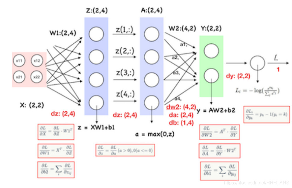
前向傳播比較簡單,就不在贅述
反向傳播需要注意的是,softmax的反向傳播與之前寫的softmax程式碼一樣。神經網路內部的反向傳播權重偏導就是前面的係數,偏置的導為1,所以就是傳播輸入的累加和,ReLU函式在反向傳播時,小於零的均為0,大於零的不變
根據求導過程可以寫出相應的程式碼,以下是具體步驟
2 - 具體步驟
構建函式,計算loss和gradients
    def loss(self, X, y=None, reg=0.0):
        """
        計算兩層全連線神經網路的loss和gradients
        輸入:
        - X :輸入維數為(N,D)
        - y : 輸入維數為(N,)
        - reg : 正則化強度

        返回:
        如果y是None,返回維數為(N,C)的分數矩陣
        如果y 不是None ,則返回一個元組:
        - loss : float 型別,資料損失和正則化損失
        - grads : 一個字典型別,儲存W1,W2,b1,b2的梯度
        """
        # Unpack variables from the params dictionary
        W1, b1 = self.params['W1'], self.params['b1']
        W2, b2 = self.params['W2'], self.params['b2']
        N, D = X.shape

        # Compute the forward pass
        scores = None

        # 完成前向傳播,並且計算loss
        # Store the result in the scores variable, which should be an array of      #
        # shape (N, C).                                                             #

        h1 = np.maximum(0, np.dot(X, W1) + b1)
        h2 = np.dot(h1, W2) + b2
        scores = h2


        # If the targets are not given then jump out, we're done

        if y is None:
            return scores

        # Compute the loss
        loss = None

        exp_class_score = np.exp(scores)
        exp_correct_class_score = exp_class_score[np.arange(N), y]

        loss = -np.log(exp_correct_class_score / np.sum(exp_class_score, axis=1))
        loss = sum(loss) / N

        loss += reg * (np.sum(W2 ** 2) + np.sum(W1 ** 2))


        # Backward pass: compute gradients
        grads = {}

        #計算反向傳播,將權重和偏置量的梯度儲存在params字典中
        # layer2
        dh2 = exp_class_score / np.sum(exp_class_score, axis=1, keepdims=True)
        dh2[np.arange(N), y] -= 1
        dh2 /= N

        dW2 = np.dot(h1.T, dh2)
        dW2 += 2 * reg * W2

        db2 = np.sum(dh2, axis=0)

        # layer1
        dh1 = np.dot(dh2, W2.T)

        dW1X_b1 = dh1
        dW1X_b1[h1 <= 0] = 0

        dW1 = np.dot(X.T, dW1X_b1)
        dW1 += 2 * reg * W1

        db1 = np.sum(dW1X_b1, axis=0)

        grads['W2'] = dW2
        grads['b2'] = db2
        grads['W1'] = dW1
        grads['b1'] = db1


        return loss, grads
完成前向和反向傳播後,其實最核心的部分就在這裡,然後我們繼續實現神經網路的訓練和預測
    def train(self, X, y, X_val, y_val,
              learning_rate=1e-3, learning_rate_decay=0.95,
              reg=5e-6, num_iters=100,
              batch_size=200, verbose=False):
        """
        使用stochastic gradient descent (SGD)來訓練神經網路
        輸入:
        -X :一個numpy陣列,維數(N,D)
        -y :一個numpy陣列,維數(N,)
        - X_val : 一個numpy陣列,維數(N_val, D)
        - y_val : 一個numpy陣列,維數(N_val,)
        - learning_rate : 學習速率
        - learning_rate_decay : 學習速率衰減
        - reg : 正則化強度
        - num_iters : 訓練次數
        - batch_size : 一批訓練的數量
        - verbose : boolean;標誌量,是否列印訓練過程
        """
        num_train = X.shape[0]
        iterations_per_epoch = max(num_train / batch_size, 1)

        # Use SGD to optimize the parameters in self.model
        loss_history = []
        train_acc_history = []
        val_acc_history = []

        for it in range(num_iters):
            X_batch = None
            y_batch = None


            # them in X_batch and y_batch respectively.
            randomIndex = np.random.choice(len(X), batch_size, replace=True)
            X_batch = X[randomIndex]
            y_batch = y[randomIndex]


            # Compute loss and gradients using the current minibatch
            loss, grads = self.loss(X_batch, y=y_batch, reg=reg)
            loss_history.append(loss)


            # Use the gradients in the grads dictionary to update the


            for param_name in self.params:
                self.params[param_name] += -learning_rate * grads[param_name]


            if verbose and it % 1000 == 0:
                print('iteration %d / %d: loss %f' % (it, num_iters, loss))

            # Every epoch, check train and val accuracy and decay learning rate.
            if it % iterations_per_epoch == 0:
                # Check accuracy
                train_acc = (self.predict(X_batch) == y_batch).mean()
                val_acc = (self.predict(X_val) == y_val).mean()
                train_acc_history.append(train_acc)
                val_acc_history.append(val_acc)

                # Decay learning rate
                learning_rate *= learning_rate_decay

        return {
            'loss_history': loss_history,
            'train_acc_history': train_acc_history,
            'val_acc_history': val_acc_history,
        }

    def predict(self, X):
        """
        使用這個網路模型的訓練權重來預測資料
        輸入:
        - X : 一個numpy陣列,維數(N,D)
        返回:
        - y_pred : 一個numpy陣列,維數(N, )
        """
        y_pred = None


        W1, b1 = self.params['W1'], self.params['b1']
        W2, b2 = self.params['W2'], self.params['b2']

        h1 = np.maximum(0, np.dot(X, W1) + b1)
        h2 = np.dot(h1, W2) + b2
        scores = h2
        y_pred = np.argmax(scores, axis=1)


        return y_pred
可以簡單的構造一個輸入資料來測試一下這個神經網路
from cs231n.classifiers.neural_net import TwoLayerNet

input_size = 4
hidden_size = 10
num_classes = 3
num_inputs = 5

def init_toy_model():
  np.random.seed(0)
  return TwoLayerNet(input_size, hidden_size, num_classes, std=1e-1)

def init_toy_data():
  np.random.seed(1)
  X = 10 * np.random.randn(num_inputs, input_size)
  y = np.array([0, 1, 2, 2, 1])
  return X, y

net = init_toy_model()
X, y = init_toy_data()

net = init_toy_model()
stats = net.train(X, y, X, y,
            learning_rate=1e-1, reg=1e-5,
            num_iters=100, verbose=False)

print('Final training loss: ', stats['loss_history'][-1])

# plot the loss history
plt.plot(stats['loss_history'])
plt.xlabel('iteration')
plt.ylabel('training loss')
plt.title('Training Loss history')
plt.show()
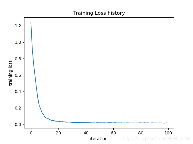
Final training loss: 0.01716153641191769
可以看到我們的網路有很好的效果,現在,就可以載入Cifar-10資料集來進行圖片的分類了。
import numpy as np
import matplotlib.pyplot as plt

from cs231n.classifiers.neural_net import TwoLayerNet
from cs231n.data_utils import load_CIFAR10


def get_CIFAR10_data(num_training=49000, num_validation=1000, num_test=1000):
  """
  將我們之前載入資料的程式碼封裝成函式
  """
  # Load the raw CIFAR-10 data
  cifar10_dir = 'cs231n/datasets/cifar-10-batches-py'
  X_train, y_train, X_test, y_test = load_CIFAR10(cifar10_dir)

  # Subsample the data
  mask = range(num_training, num_training + num_validation)
  X_val = X_train[mask]
  y_val = y_train[mask]
  mask = range(num_training)
  X_train = X_train[mask]
  y_train = y_train[mask]
  mask = range(num_test)
  X_test = X_test[mask]
  y_test = y_test[mask]

  # Normalize the data: subtract the mean image
  mean_image = np.mean(X_train, axis=0)
  X_train -= mean_image
  X_val -= mean_image
  X_test -= mean_image

  # Reshape data to rows
  X_train = X_train.reshape(num_training, -1)
  X_val = X_val.reshape(num_validation, -1)
  X_test = X_test.reshape(num_test, -1)

  return X_train, y_train, X_val, y_val, X_test, y_test

# 載入資料集
X_train, y_train, X_val, y_val, X_test, y_test = get_CIFAR10_data()
input_size = 32 * 32 * 3
hidden_size = 50
num_classes = 10
net = TwoLayerNet(input_size, hidden_size, num_classes)

# Train the network
stats = net.train(X_train, y_train, X_val, y_val,
            num_iters=3000, batch_size=200,
            learning_rate=1e-4, learning_rate_decay=0.95,
            reg=0.5, verbose=True)

# Predict on the validation set
val_acc = (net.predict(X_val) == y_val).mean()
print('Validation accuracy: ', val_acc)

# Plot the loss function and train / validation accuracies
plt.subplot(2, 1, 1)
plt.plot(stats['loss_history'])
plt.title('Loss history')
plt.ylabel('Loss')

plt.subplot(2, 1, 2)
plt.plot(stats['train_acc_history'], label='train')
plt.plot(stats['val_acc_history'], label='val')
plt.xlabel('Epoch')
plt.ylabel('Clasification accuracy')
plt.show()
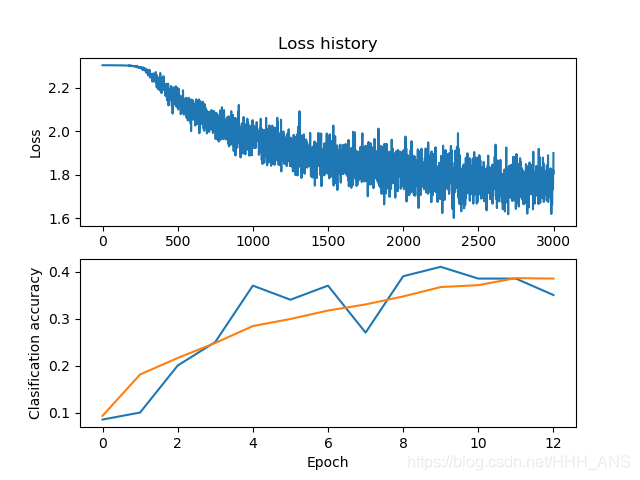
iteration 0 / 3000: loss 2.303370
iteration 1000 / 3000: loss 2.050751
iteration 2000 / 3000: loss 1.816003
Validation accuracy:  0.39
可以看到使用初始設定的超引數準確率只有39%,所以我們接下來需要使用交叉驗證來尋找最適合的超引數。
# 載入資料集
X_train, y_train, X_val, y_val, X_test, y_test = get_CIFAR10_data()
input_size = 32 * 32 * 3
num_classes = 10
best_net = None # store the best model into this
hidden_size = [75, 100, 125]

results = {}
best_val_acc = 0
best_net = None

learning_rates = np.array([0.7, 0.8, 0.9, 1, 1.1]) * 1e-3
regularization_strengths = [0.75, 1, 1.25]

print('running')
for hs in hidden_size:
  for lr in learning_rates:
    for reg in regularization_strengths:
      print(',')
      net = TwoLayerNet(input_size, hs, num_classes)
      # Train the network
      stats = net.train(X_train, y_train, X_val, y_val,
                        num_iters=1500, batch_size=200,
                        learning_rate=lr, learning_rate_decay=0.95,
                        reg=reg, verbose=False)
      val_acc = (net.predict(X_val) == y_val).mean()
      if val_acc > best_val_acc:
        best_val_acc = val_acc
        best_net = net
      results[(hs, lr, reg)] = val_acc
print()
print("finshed")
# Print out results.
for hs, lr, reg in sorted(results):
  val_acc = results[(hs, lr, reg)]
  print('hs %d lr %e reg %e val accuracy: %f' % (hs, lr, reg, val_acc))

print('best validation accuracy achieved during cross-validation: %f' % best_val_acc)
輸出結果如下,經過交叉驗證之後準確率提升到了49%,接近50%
hs 75 lr 7.000000e-04 reg 7.500000e-01 val accuracy: 0.465000
hs 75 lr 7.000000e-04 reg 1.000000e+00 val accuracy: 0.466000
hs 75 lr 7.000000e-04 reg 1.250000e+00 val accuracy: 0.451000
hs 75 lr 8.000000e-04 reg 7.500000e-01 val accuracy: 0.458000
hs 75 lr 8.000000e-04 reg 1.000000e+00 val accuracy: 0.479000
hs 75 lr 8.000000e-04 reg 1.250000e+00 val accuracy: 0.462000
hs 75 lr 9.000000e-04 reg 7.500000e-01 val accuracy: 0.469000
hs 75 lr 9.000000e-04 reg 1.000000e+00 val accuracy: 0.462000
hs 75 lr 9.000000e-04 reg 1.250000e+00 val accuracy: 0.468000
hs 75 lr 1.000000e-03 reg 7.500000e-01 val accuracy: 0.487000
hs 75 lr 1.000000e-03 reg 1.000000e+00 val accuracy: 0.467000
hs 75 lr 1.000000e-03 reg 1.250000e+00 val accuracy: 0.470000
hs 75 lr 1.100000e-03 reg 7.500000e-01 val accuracy: 0.479000
hs 75 lr 1.100000e-03 reg 1.000000e+00 val accuracy: 0.476000
hs 75 lr 1.100000e-03 reg 1.250000e+00 val accuracy: 0.473000
hs 100 lr 7.000000e-04 reg 7.500000e-01 val accuracy: 0.476000
hs 100 lr 7.000000e-04 reg 1.000000e+00 val accuracy: 0.475000
hs 100 lr 7.000000e-04 reg 1.250000e+00 val accuracy: 0.458000
hs 100 lr 8.000000e-04 reg 7.500000e-01 val accuracy: 0.486000
hs 100 lr 8.000000e-04 reg 1.000000e+00 val accuracy: 0.477000
hs 100 lr 8.000000e-04 reg 1.250000e+00 val accuracy: 0.464000
hs 100 lr 9.000000e-04 reg 7.500000e-01 val accuracy: 0.490000
hs 100 lr 9.000000e-04 reg 1.000000e+00 val accuracy: 0.479000
hs 100 lr 9.000000e-04 reg 1.250000e+00 val accuracy: 0.476000
hs 100 lr 1.000000e-03 reg 7.500000e-01 val accuracy: 0.495000
hs 100 lr 1.000000e-03 reg 1.000000e+00 val accuracy: 0.469000
hs 100 lr 1.000000e-03 reg 1.250000e+00 val accuracy: 0.472000
hs 100 lr 1.100000e-03 reg 7.500000e-01 val accuracy: 0.483000
hs 100 lr 1.100000e-03 reg 1.000000e+00 val accuracy: 0.470000
hs 100 lr 1.100000e-03 reg 1.250000e+00 val accuracy: 0.459000
hs 125 lr 7.000000e-04 reg 7.500000e-01 val accuracy: 0.473000
hs 125 lr 7.000000e-04 reg 1.000000e+00 val accuracy: 0.478000
hs 125 lr 7.000000e-04 reg 1.250000e+00 val accuracy: 0.466000
hs 125 lr 8.000000e-04 reg 7.500000e-01 val accuracy: 0.467000
hs 125 lr 8.000000e-04 reg 1.000000e+00 val accuracy: 0.483000
hs 125 lr 8.000000e-04 reg 1.250000e+00 val accuracy: 0.471000
hs 125 lr 9.000000e-04 reg 7.500000e-01 val accuracy: 0.481000
hs 125 lr 9.000000e-04 reg 1.000000e+00 val accuracy: 0.480000
hs 125 lr 9.000000e-04 reg 1.250000e+00 val accuracy: 0.479000
hs 125 lr 1.000000e-03 reg 7.500000e-01 val accuracy: 0.471000
hs 125 lr 1.000000e-03 reg 1.000000e+00 val accuracy: 0.479000
hs 125 lr 1.000000e-03 reg 1.250000e+00 val accuracy: 0.458000
hs 125 lr 1.100000e-03 reg 7.500000e-01 val accuracy: 0.474000
hs 125 lr 1.100000e-03 reg 1.000000e+00 val accuracy: 0.470000
hs 125 lr 1.100000e-03 reg 1.250000e+00 val accuracy: 0.469000
best validation accuracy achieved during cross-validation: 0.495000