有些情況,  我們會需要提取直線的詳細引數, 下面介紹如何提取直線

霍夫變換(Hough Transformation)

其中很大一部分都在應用霍夫變換 及其 各種版本來提取直線

     這裡個人總結下:  霍夫變換的基本思想,   將原本的平面曲線引數方程轉化成 , 以曲線上點作為已知,

把曲線方程的引數當作未知項,  在引數空間作出圖形.(原本已知所有引數時可以求出曲線上的這些點)

     當交於某公共點上圖形最多時(peak),  這個公共點(peak)對應的引數便可作為整個圖形的引數.

霍夫變換最開始提出來時,  直線方程用的是斜截式

       因為考慮到直線兩種極端情況,  水平和豎直

所以按斜率是否大於1,  使用了不同的方程

       k < 1 時       y = kx +b

       k>=1 時       y = 1/k x + 1/b  

就避免了因為 y = mx + c   中  m,c 過大而不好討論(m,c代表直線方程的引數)

        ρ = x cos θ + y sin θ
來表示直線,  也就是現在常見的表示形式

提供了減少計算量的方法

最好看看hough變換的原始碼,  因為opencv只提供了直線和圓的函式,  其他的需要自己去寫

下面示例下opencv霍夫變換函式的使用

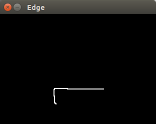
注: sobel運算元使用的方法不太正確, 這裡僅作示例用. 兩圖求得的edge不一樣

cv::MatG,Gx,Gy,G_otsu;

cv::Sobel(srcEmpty,Gx,CV_8U,1,0,3);

cv::Sobel(srcEmpty,Gy,CV_8U,0,1,3);

G=Gx+Gy;

cv::threshold(G,G_otsu,0,255,cv::THRESH_OTSU);

if(debugflag)

cv::imshow("Edge",G_otsu);

cv::Matdst(srcEmpty.size(),CV_8UC3);

std::vector<cv::Vec2f>lines;

cv::HoughLines(G_otsu,lines,1,CV_PI
 
/180,30,0,0);

for(size_ti=0;i<lines.size();i++){

floatrho=lines[i][0];

floattheta=lines[i][1];

doublea=cos(theta),b=sin(theta);

doublex0=a*rho,y0=b*rho;

cv::Pointpt1(cvRound(x0+1000*(-b)),cvRound(y0+1000*(a)));

cv::Pointpt2(cvRound(x0-1000*(-b)),cvRound(y0-1000*(a)));

cv::line(dst,pt1,pt2,cv::Scalar(0,0,255),3,8);

}

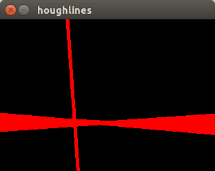
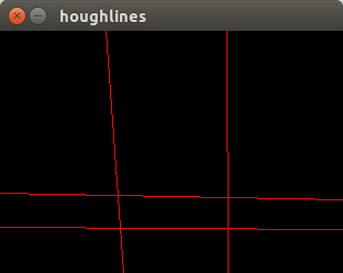
可以看到,  找出的直線並沒有邊界(直線的兩端點)

至於為什麼會出現右圖多條直線的那種情況

因為用於投票的閾值 

太高只能提取長線, 短線被忽略

太低又會出現多條,  這種情況,  不好確定閾值

這個時候如果單單是呼叫houghLines的話,  可能不會有太好的結果

再來看houghLinesP的使用

std::vector<cv::Vec4i>lines;

cv::HoughLinesP(srcEmpty,lines,1,CV_PI/180,20,20,20);

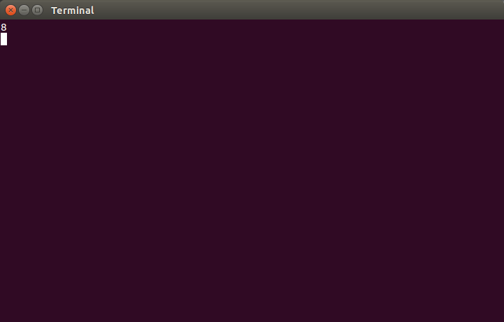
std::cout<<lines.size()<<std::endl;

for(size_ti=0;i<lines.size();i++){

cv::line(dst,cv::Point(lines[i][0],lines[i][1]),

cv::Point(lines[i][2],lines[i][3]),cv::Scalar(0,0,255),3,8);

}

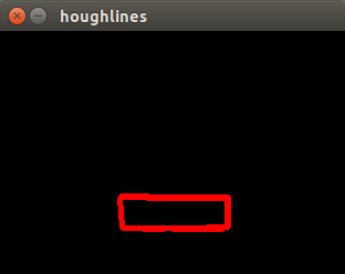
看起來好多了.但是我們看看本意提取的四條線 

cout << line.size() 的結果是8條

而且選定的引數也僅僅是針對這個邊緣,  稍微變化一點引數又要變化

可以的話,  對兩端點之內相交的線段,  定義夾角範圍多少以內是同一條邊,  

在這些邊選取最長的線段作為整條邊

對於本情況,  需要的並不是提取所有直線,  而是根據這個edge的特點,  找到四條滿足大部分點的直線

因此,  opencv所提供的兩個霍夫變換並不適合這種情況

(重點在對邊緣直線長度未知的情況下,  沒有很好的引數適用大部分情況)

需要對函式根據需要進行一些修改

例如

原圖:   

結果:   

注 :  改動部分為   由返回符合threshold的多條直線,   變為    返回獲得票數最高的直線

RANSAC

在opencv中,  涉及到ransac的函式只有跟立體標定有關

所以想直接調函式的還是不要想opencv了吧

本人所寫的ransac 函式,  僅供參考 ,  傳送門:  我的github

http://www.cnblogs.com/xrwang/archive/2011/03/09/ransac-1.html

http://grunt1223.iteye.com/blog/961063

關於RANSAC c++程式碼    很抱歉這裡沒有進行實驗,  請自行甄別

https://github.com/srinath1905/GRANSAC/blob/master/include/GRANSAC.hpp

http://reference.mrpt.org/stable/classmrpt_1_1math_1_1_r_a_n_s_a_c___template.html 及

https://github.com/MRPT/mrpt/blob/9f72d70abe8db107f7331f3723cf2553d7c307d0/libs/base/include/mrpt/math/ransac.h

https://github.com/MRPT/mrpt/blob/9f72d70abe8db107f7331f3723cf2553d7c307d0/libs/base/src/math/ransac.cpp

  及

http://www.mrpt.org/tutorials/programming/maths-and-geometry/ransac-c-examples/

    要使用RANSAC擬合直線,  我們首先需要三個引數

1.The Number of Samples Required

    假設我們需要畫n個點(對於擬合直線來說, 最少需要兩個點; 對於圓則最少需要三個.),  

其中w是其中好點(good points, 有效點?)所佔的比例,  

則需要畫的次數(the number of draws k)的期望值是     

                                                          E[k] = w ^ (-n)

                        

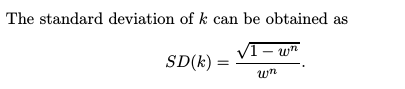
             假設當只有bad samples 出現的概率為 z

                                         則

                                                 

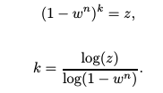
這三種方法都可以求出k

其中每個sample裡面包括the abstraction of interest所需要的最少點. 

2.Telling Whether a Point Is Close                  距離直線的最大距離的點

3.The Number of Points That Must Agree       (在前面所確定的距離內) 需要最少個數的點

    對於本情況,  對四條線段使用 RANSAC,  具體的想法是:

1.  對一組點集用投票法找出最高票數的直線,  找出peak後並刪掉peak對應的資料

2.  找出下一條直線,   同樣找出並刪除對應的資料

3.  就這樣迴圈,  直到找出4條直線,  終止

  

來源: computer vision : a modern approatch

擬合法

   相對於RANSAC對噪聲不敏感,  因為擬合法是對當前所有的點進行的, 內在並沒有一個檢測和去除

壞點(gross point)的機制[Matin and Robert, 1980],  除了提供儘可能大的相關資料外

使用擬合法之前一定要把儘量無關的點去除

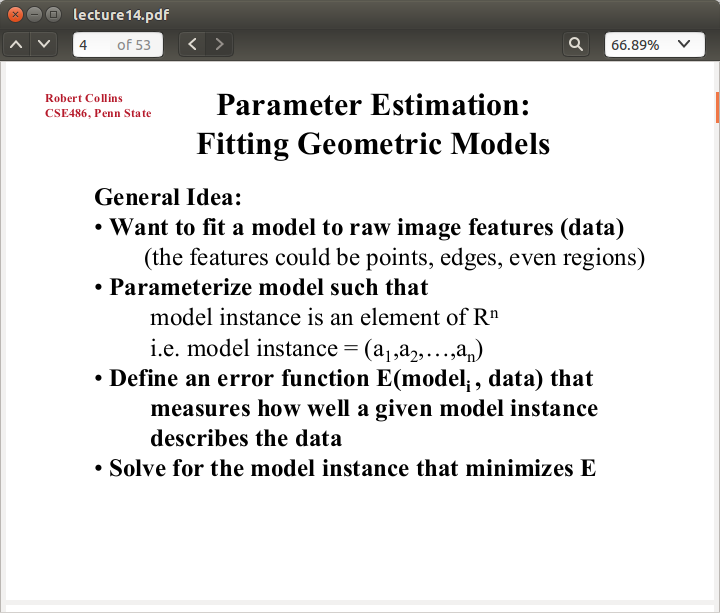
    擬合法在前面常提的課件(www.cse.psu.edu) , lecture14 有講,  

以最小二乘法為例

比如直線點斜式方程

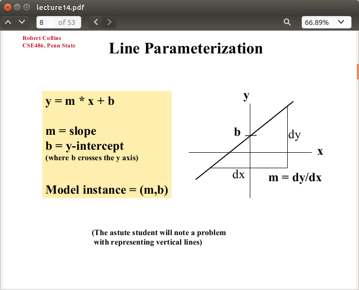
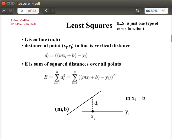
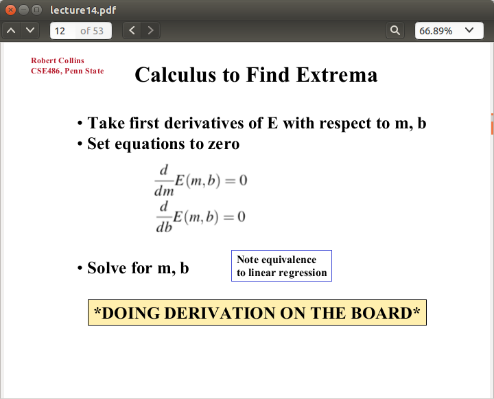
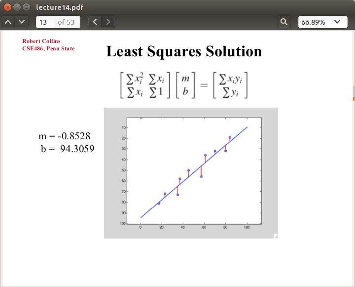
圖片來源:  http://www.cse.psu.edu/~rtc12/CSE486/

對於直線一般方程,  一樣的原理,  

ax+ by +c = 0 = d0

di = axi + byi +c

E(a,b,c) = ⅀ (di - d0 ) ^2

求導 ,  令導數為0,   就得到了 可以求解(a,b,c) 方程組

注意當所有點都在同一條直線上時,  方程組的引數矩陣的一個特徵值為0,  此時齊次方程有無數多的解.

詳細請自尋

opencv提供了直線擬合法函式fitLine(),  我用的3.1.0 調了很久都沒有調通,  高度懷疑此處存在bug,具體點選這裡

fitLine原始碼在下面,後面列出了引數參考

     用上面的存放edge影象的Mat時會出現

OpenCV Error: Assertion failed (npoints2 >= 0 || npoints3 >= 0) in fitLine,

 file /home/tau/opencv/opencv-3.1.0/modules/imgproc/src/linefit.cpp, line 603
terminate called after throwing an instance of 'cv::Exception'
  what():  /home/tau/opencv/opencv-3.1.0/modules/imgproc/src/linefit.cpp:603: 

error: (-215) npoints2 >= 0 || npoints3 >= 0 in function fitLine

    哪裡出了問題呢?  我們來試試看看fitLine原始碼吧,  原始碼在下面

opencv 3.0 對這一部分用c++ 重寫了一遍,  當然這裡呼叫了c函式的FitLine2D, 這裡不去深究

在這個函式發現錯誤提示來自這裡

CV_Assert( npoints2 >= 0 || npoints3 >= 0

而int npoints2 = points.checkVector(2, -1, false);

函式的功能是: 當Mat的channels,depth,和連續性  滿足checkVector的引數內容時,

返回(int)(total()*channels()/_elemChannels), 否則返回-1

看出問題沒有? 

因為存放edge的Mat是連續的, 而checkVector(2,-1,false)要求是不連續的, 所以被返回了-1

且npoints2與npoints3 都被返回了-1

怎麼解決呢?

首先肯定要想怎麼把畫素值不為0的點提取出來, 存成vector或Mat,

用findContours之類的. 或是乾脆自己將edge分成四段線段,這樣也避免了四條線相互影響

    雖然對於上面的edge四條線段確實可以用四條直線擬合,  

但是我還沒有想好怎麼方便把四條線段上的點分別存放, 以便直接使用fitLine

既然想到了findContours,  那就是把存放edge的Mat資料的非零點存成點集.

    在這裡,  我先用了角點檢測將完整的edge打斷成四條線段,  但是不知道什麼原因fitline函式總是無法正常執行

所以等到解決後再更新本文吧

關於points.checkVector()    

int cv::Mat::checkVector	(	int	elemChannels,
int	depth = -1,
bool	requireContinuous = true
)	const

returns N if the matrix is 1-channel (N x ptdim) or ptdim-channel (1 x N) or (N x 1); negative number otherwise

雖然未對depth與requireContinuous進行說明,但從命名上看應該能看明白吧

int Mat::checkVector(int _elemChannels, int _depth, bool _requireContinuous) const
{
    return (depth() == _depth || _depth <= 0) &&  (isContinuous() || !_requireContinuous) &&
               ((dims == 2 && (((rows == 1 || cols == 1) && channels() == _elemChannels) ||(cols == _elemChannels && channels() == 1))) ||
        (dims == 3 && channels() == 1 && size.p[2] == _elemChannels && (size.p[0] == 1 || size.p[1] == 1) &&
         (isContinuous() || step.p[1] == step.p[2]*size.p[2])))
    ? (int)(total()*channels()/_elemChannels) : -1;
}

void cv::fitLine( InputArray _points, OutputArray _line, int distType, double param, double reps, double aeps )
{
    Mat points = _points.getMat();
    float linebuf[6]={0.f};
    int npoints2 = points.checkVector(2, -1, false);
    int npoints3 = points.checkVector(3, -1, false);
    CV_Assert( npoints2 >= 0 || npoints3 >= 0 );
    if( points.depth() != CV_32F || !points.isContinuous() )
    {
        Mat temp;
        points.convertTo(temp, CV_32F);
        points = temp;
    }
    if( npoints2 >= 0 )
        fitLine2D( points.ptr<Point2f>(), npoints2, distType, (float)param, (float)reps, (float)aeps, linebuf);
    else
        fitLine3D( points.ptr<Point3f>(), npoints3, distType, (float)param, (float)reps, (float)aeps, linebuf);
    Mat(npoints2 >= 0 ? 4 : 6, 1, CV_32F, linebuf).copyTo(_line);
}

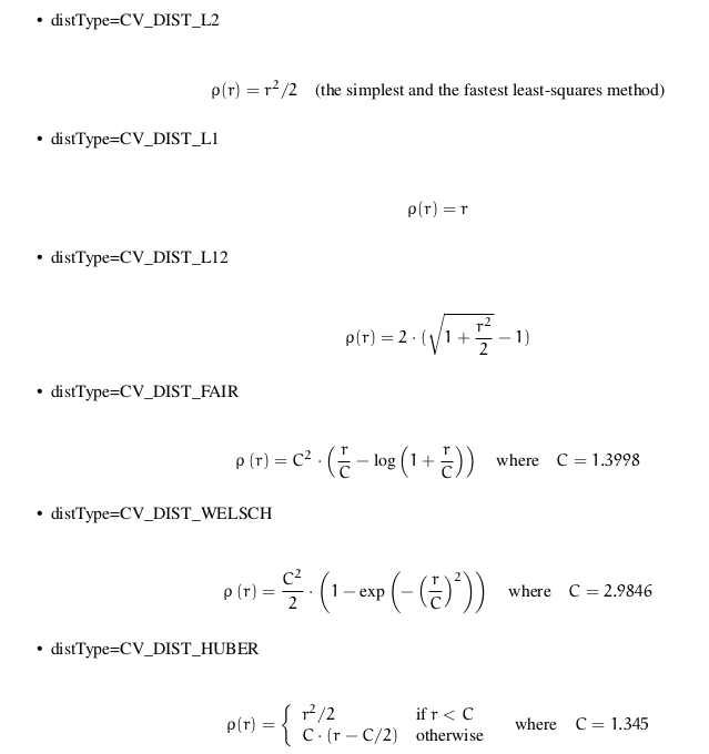
其中distType可選引數

Parameters

points	Input vector of 2D or 3D points, stored in std::vector<> or Mat.
line	Output line parameters. In case of 2D fitting, it should be a vector of 4 elements (like Vec4f) - (vx, vy, x0, y0), where (vx, vy) is a normalized vector collinear to the line and (x0, y0) is a point on the line. In case of 3D fitting, it should be a vector of 6 elements (like Vec6f) - (vx, vy, vz, x0, y0, z0), where (vx, vy, vz) is a normalized vector collinear to the line and (x0, y0, z0) is a point on the line.
distType	Distance used by the M-estimator, see cv::DistanceTypes
param	Numerical parameter ( C ) for some types of distances. If it is 0, an optimal value is chosen.
reps	Sufficient accuracy for the radius (distance between the coordinate origin and the line).
aeps	Sufficient accuracy for the angle. 0.01 would be a good default value for reps and aeps.

void HoughLines( InputArray image, OutputArray lines, double rho, double theta, int threshold, double srn=0, 

                                                                                         double stn=0 )

image – 8-bit, single-channel binary source image. The image may be modified by the function.

lines –   Output vector of lines. Each line is represented by a two-element vector (ρ, θ) . 

              ρ is the distance from the coordinate origin (0, 0) (top-left corner of the image). θ is the line

              rotation angle in radians ( 0 ∼ vertical line, π/2 ∼ horizontal line ).

rho –      Distance resolution of the accumulator in pixels.

theta –    Angle resolution of the accumulator in radians.

threshold – Accumulator threshold parameter. Only those lines are returned that get enough votes ( > threshold ).

srn – For the multi-scale Hough transform, it is a divisor for the distance resolution rho .

         The coarse accumulator distance resolution is rho and the accurate accumulator resolution
         is rho/srn . If both srn=0 and stn=0 , the classical Hough transform is used. Otherwise,
         both these parameters should be positive.

stn – For the multi-scale Hough transform, it is a divisor for the distance resolution theta .

method – One of the following Hough transform variants:

– CV_HOUGH_STANDARD classical or standard Hough transform. Every line is repre-
sented by two floating-point numbers (ρ, θ) , where ρ is a distance between (0,0) point
and the line, and θ is the angle between x-axis and the normal to the line. Thus, the matrix
must be (the created sequence will be) of CV_32FC2 type

– CV_HOUGH_PROBABILISTIC probabilistic Hough transform (more efficient in case
if the picture contains a few long linear segments). It returns line segments rather than
the whole line. Each segment is represented by starting and ending points, and the matrix
must be (the created sequence will be) of the CV_32SC4 type.

– CV_HOUGH_MULTI_SCALE multi-scale variant of the classical Hough transform.
The lines are encoded the same way as CV_HOUGH_STANDARD .

void HoughLinesP( InputArray image, OutputArray lines, double rho, double theta, int threshold, 

                                                                 double minLineLength=0, double maxLineGap=0 )

image – 8-bit, single-channel binary source image. The image may be modified by the function.

lines – Output vector of lines. Each line is represented by a 4-element vector (x 1 , y 1 , x 2 , y 2 ),

where (x 1 , y 1 ) and (x 2 , y 2 ) are the ending points of each detected line segment.

rho – Distance resolution of the accumulator in pixels.

theta – Angle resolution of the accumulator in radians.

threshold – Accumulator threshold parameter. Only those lines are returned that get enough votes ( > threshold ).

minLineLength – Minimum line length. Line segments shorter than that are rejected.

maxLineGap – Maximum allowed gap between points on the same line to link them.

今天接觸到LSD演算法  http://blog.csdn.net/carson2005/article/details/9326847   改天增加這部分內容

http://docs.opencv.org/master/d1/dbd/classcv_1_1line__descriptor_1_1LSDDetector.html#gsc.tab=0